InDetail2-DataExploration • finnsurveytext

Introduction

Exploratory Data Analysis (EDA) is a common activity once data has been cleaned and prepared. EDA involves running functions which allow you to better understand the responses and begin to formulate initial hypotheses based on the data.

This tutorial follows on from Tutorial 1 and guides you through an EDA of data which has been prepared into CoNLL-U format. These EDA functions are contained in r/02_data_exploration.R.

Installation of package.

Once the package is installed, you can load the finnsurveytext package as below: (Other required packages such as dplyr and stringr will also be installed if they are not currently installed in your environment.)

library(finnsurveytext)

Overview of Functions

The functions covered in this tutorial are:

Data

There are two sets of data files available within the package which could be used in this tutorial. These files have been created following the process demonstrated in Tutorial 1.

1. Child Barometer Data

data/fst_child.rda

2. Development Cooperation Data

data/fst_dev_coop

You can read these in as follows:

df1 <- fst_child
df2 <- fst_dev_coop

Summary Tables

Get Summary Table functions

fst_summarise_short() and fst_summarise()

This first function creates a simple summary table for the data that shows the total number of words, number of unique words, and number of unique lemmas in the data. You can either view the table in the console, or define a variable which will contain this table.

The second function adds information about the number and proportion of survey respondents which answered this question.

fst_summarise_short(data = df1)
#>   Respondents Total Words Unique Words Unique Lemmas
#> 1         413        1580          559           414

summary_table <- fst_summarise(data = df2, desc = "All")
knitr::kable(summary_table)

Description	Respondents	No Response	Proportion	Total Words	Unique Words	Unique Lemmas
All	945	25	0.97	4192	1132	994

fst_summarise_short() and fst_summarise() take 1 argument:

data is output from data preparation, prepared data in CoNLL-U format, such as the output of fst_prepare_connlu().

fst_summarise() takes an optional second argument:

desc is an optional string describing respondents. This description is included in the table in the first column. If not defined, it will default to ‘All respondents’.

Get Part-Of-Speech Summary Table function

fst_pos()

This function creates a table which counts the number and proportion of words of each part-of-speech (POS) tag within the data. Again, you can either view the table in the console, or define a variable which will contain this table.

fst_pos(data = df1)
#>     UPOS                  UPOS_Name Count Proportion
#> 1    ADJ                  adjective   156      0.099
#> 2    ADP                 adposition     5      0.003
#> 3    ADV                     adverb    98      0.062
#> 4    AUX                  auxiliary    36      0.023
#> 5  CCONJ   coordinating conjunction     1      0.001
#> 6    DET                 determiner    72      0.046
#> 7   INTJ               interjection    16      0.010
#> 8   NOUN                       noun   455      0.288
#> 9    NUM                    numeral     2      0.001
#> 10  PART                   particle    38      0.024
#> 11  PRON                    pronoun   148      0.094
#> 12 PROPN                proper noun     6      0.004
#> 13 PUNCT                punctuation    NA         NA
#> 14 SCONJ  subordinating conjunction    NA         NA
#> 15   SYM                     symbol    NA         NA
#> 16  VERB                       verb   545      0.345
#> 17     X                      other     2      0.001

pos_table <- fst_pos(data = df2)
knitr::kable(pos_table)

UPOS	UPOS_Name	Count	Proportion
ADJ	adjective	389	0.093
ADP	adposition	24	0.006
ADV	adverb	64	0.015
AUX	auxiliary	3	0.001
CCONJ	coordinating conjunction	3	0.001
DET	determiner	28	0.007
INTJ	interjection	2	0.000
NOUN	noun	3311	0.790
NUM	numeral	5	0.001
PART	particle	29	0.007
PRON	pronoun	12	0.003
PROPN	proper noun	31	0.007
PUNCT	punctuation	NA	NA
SCONJ	subordinating conjunction	NA	NA
SYM	symbol	1	0.000
VERB	verb	278	0.066
X	other	12	0.003

fst_pos() takes 1 argument:

data is output from data preparation, prepared data in CoNLL-U format, such as the output of fst_prepare_connlu().

Get Length Summary Table function

fst_length_summary()

This function creates a table which summarises the distribution of lengths in the responses. Again, you can either view the table in the console, or define a variable which will contain this table.

fst_length_summary(data = df1, desc = "All Children")
#> # A tibble: 2 × 8
#>   Description             Respondents  Mean Minimum    Q1 Median    Q3 Maximum
#>   <chr>                         <int> <dbl>   <int> <dbl>  <int> <dbl>   <int>
#> 1 All Children- Words             413  5.33       1     2      4     7      37
#> 2 All Children- Sentences         413  1.22       1     1      1     1       6

length_table <- fst_length_summary(data = df2, incl_sentences = FALSE)
knitr::kable(length_table)

Description	Respondents	Mean	Minimum	Q1	Median	Q3	Maximum
All responses- Words	920	5.515	1	4	5	6	32

fst_length_summary() takes 3 arguments:

data is output from data preparation, prepared data in CoNLL-U format, such as the output of fst_prepare_connlu().
desc is an optional string describing respondents. If not defined, it will remain blank in the table meaning that the ‘Description’ column will only show whether the row is showing data for words or sentences.
incl_sentences is a boolean of whether to include sentence data in table, default is TRUE. If incl_sentences = TRUE, the table will also provide length information for the number of sentences within responses. If incl_sentences = FALSE, the table will show only show results for the number of words in responses.

Top Words and N-grams Tables

Next we will demonstrate some functions which are used to create plots of most frequent words and n-grams occurring in the data. An n-gram is a set of n successive words in the data.

Make Top Words Table function

fst_freq_table()

This functions creates a table of the most frequently occurring words in the data (noting that “stopwords” may have been removed in previous data preparation steps.)

The top words tables is able have the words normalised if you choose. The variable norm is the method for normalising the data. Valid settings are 'number_words' (the number of words in the responses), 'number_resp' (the number of responses), or NULL (raw count returned, default).

Optionally, you can indicate which POS tags to include.

In this function, you must determine what you want to do in the case of ties with the variable strict. Words with equal occurrence are presented in alphabetial order. By default, words are presented in order to the number cutoff word. This means that equally-occurring later-alphabetically words beyond the cutoff word will not be displayed. Alternatively, you can decide that the cutoff is not strict, in which case words occurring equally often as the number cutoff words will be displayed. (fst_freq_table() will print a message regarding this decision.)

We run the functions as follows:

fst_freq_table(data = df1)
#> Note:
#>  Words with equal occurrence are presented in alphabetical order. 
#>  By default, words are presented in order to the `number` cutoff word. 
#>  This means that equally-occurring later-alphabetically words beyond the cutoff word will not be displayed.
#>       words occurrence
#> 1    toinen        118
#> 2     lyödä         71
#> 3  lyöminen         53
#> 4      joku         46
#> 5      paha         43
#> 6     tehdä         34
#> 7     sanoa         33
#> 8    tietää         32
#> 9     jokin         30
#> 10    tulla         30

fst_freq_table(
  data = df1,
  number = 15,
  norm = NULL,
  pos_filter = c("NOUN", "VERB", "ADJ", "ADV"),
  strict = FALSE, 
  use_svydesign_weights = FALSE,
  id = "",
  svydesign = NULL,
  use_column_weights = FALSE
)
#> Note:
#>  Words with equal occurrence are presented in alphabetical order. 
#>  With `strict` = FALSE, words occurring equally often as the `number` cutoff word will be displayed.
#>         words occurrence
#> 1       lyödä         71
#> 2    lyöminen         53
#> 3        paha         42
#> 4       sanoa         33
#> 5       tehdä         33
#> 6      tietää         32
#> 7       tulla         29
#> 8       ottaa         28
#> 9      potkia         27
#> 10    kiusata         26
#> 11 potkiminen         24
#> 12    haukkua         22
#> 13     kaveri         22
#> 14  töniminen         22
#> 15     toinen         17
#> 16      tyhmä         17
#> 17      tönia         17
                           

table1 <- fst_freq_table(data = df2, number = 5)
#> Note:
#>  Words with equal occurrence are presented in alphabetical order. 
#>  By default, words are presented in order to the `number` cutoff word. 
#>  This means that equally-occurring later-alphabetically words beyond the cutoff word will not be displayed.
knitr::kable(table1)

words	occurrence
köyhyys	258
nälänhätä	239
sota	231
ilmastonmuutos	141
puute	117


table2 <- fst_freq_table(data = df2, number = 5, norm = "number_resp", pos_filter = c("NOUN", "VERB"), strict = FALSE)
#> Note:
#>  Words with equal occurrence are presented in alphabetical order. 
#>  With `strict` = FALSE, words occurring equally often as the `number` cutoff word will be displayed.
knitr::kable(table2)

words	occurrence
köyhyys	0.273
nälänhätä	0.253
sota	0.244
ilmastonmuutos	0.149
puute	0.124

fst_freq_table() takes the following arguments:

data is output from data preparation, prepared data in CoNLL-U format, such as the output of fst_prepare_connlu().
number is the number of top words/n-grams to return, default is 10 which means that the top 10 words will be returned.
norm is the method for normalising the data. Valid settings are 'number_words' (the number of words in the responses), 'number_resp' (the number of responses), or NULL (raw count returned, default).
pos_filter is an optional list of which POS tags to include such as 'c("NOUN", "VERB", "ADJ", "ADV")'. The default is NULL, in which case all words in the data are considered.
strict is a boolean that determines how the function will deal with ‘ties’. If strict = TRUE, the table will cut-off at the exact number(words are presented in alphabetical order so later-alphabetically, equally occurring words to the word at number will not be shown.) If strict = FALSE, the table will show any words that occur equally frequently as the number cutoff word.
use_svydesign_weights is a boolean for whether to get weights for the responses from a svydesign object
If weights are coming from a svydesign object, the id field needs to not be empty, as this is used to join the data.
Similarly, if weights are coming from a svydesign object this is the named object.
use_column_weights is a boolean for if weights have already been included in the formatted data and should be included.

Make Top N-Grams Table function

fst_ngrams_table()

Similar to fst_freq_table(), this functions creates a table of the most frequently occurring n-grams in the data (noting that “stopwords” may have been removed in previous data preparation steps.)

The top n-grams tables are able have the n-grams normalised if you choose. The variable norm is the method for normalising the data. Valid settings are 'number_words' (the number of words in the responses), 'number_resp' (the number of responses), or NULL (raw count returned, default).

Optionally, you can indicate which POS tags to include.

In this function, you must determine what you want to do in the case of ties with the variable strict. N-grams with equal occurrence are presented in alphabetial order. By default, n-grams are presented in order to the number cutoff n-gram. This means that equally-occurring later-alphabetically n-grams beyond the cutoff n-gram will not be displayed. Alternatively, you can decide that the cutoff is not strict, in which case n-grams occurring equally often as the number cutoff n-gram will be displayed. (fst_get_top_ngrams() will print a message regarding this decision. There is another function fst_ngrams_table2() which doesn’t print a message. This function is used within the comparison functions in 04_comparison_functions.R)

We run the functions as follows:

fst_ngrams_table(data = df1, ngrams = 2)
#> Note:
#>  N-grams with equal occurrence are presented in alphabetical order. 
#>  By default, n-grams are presented in order to the `number` cutoff n-gram. 
#>  This means that equally-occurring later-alphabetically n-grams beyond the cutoff n-gram will not be displayed.
#>                  words occurrence
#> 1  lyöminen potkiminen         17
#> 2           joku lyödä         11
#> 3         lyödä potkia         11
#> 4          osata sanoa          9
#> 5       haukkua toinen          8
#> 6          sanoa jokin          7
#> 7          tulla mieli          7
#> 8          joku toinen          6
#> 9         ottaa toinen          6
#> 10          paha mieli          6

fst_ngrams_table(data = df1, ngrams = 2, norm = "number_words", strict = FALSE)
#> Note:
#>  N-grams with equal occurrence are presented in alphabetical order. 
#>  With `strict` = FALSE, n-grams occurring equally often as the `number` cutoff n-gram will be displayed.
#>                  words occurrence
#> 1  lyöminen potkiminen      0.011
#> 2           joku lyödä      0.007
#> 3         lyödä potkia      0.007
#> 4          osata sanoa      0.006
#> 5       haukkua toinen      0.005
#> 6          sanoa jokin      0.004
#> 7          tulla mieli      0.004
#> 8          joku toinen      0.004
#> 9         ottaa toinen      0.004
#> 10          paha mieli      0.004
#> 11     pyytää anteeksi      0.004
#> 12         tehdä jokin      0.004
#> 13        tietää lyödä      0.004
#> 14        toinen tulla      0.004
#> 15  töniminen lyöminen      0.004

table3 <- fst_ngrams_table(data = df2, number = 15, ngrams = 3)
#> Note:
#>  N-grams with equal occurrence are presented in alphabetical order. 
#>  By default, n-grams are presented in order to the `number` cutoff n-gram. 
#>  This means that equally-occurring later-alphabetically n-grams beyond the cutoff n-gram will not be displayed.
knitr::kable(table3)

words	occurrence
puhdas vesi puute	38
nälänhätä puhdas vesi	9
nälkä puhdas vesi	7
puhdas juomavesi puute	6
epätasainen jakautuminen ilmastonmuutos	5
köyhyys nälänhätä sota	5
köyhyys puhdas vesi	5
nälänhätä sota eriarvoisuus	5
varallisuus epätasainen jakautuminen	5
vesi puute sota	5
nainen huono asema	4
nälkä köyhyys sota	4
nälänhätä ihminen itsekkyys	4
nälänhätä sota nälänhätä	4
sota köyhyys nälänhätä	4


table4 <- fst_ngrams_table(data = df2, number = 15, ngrams = 2, pos_filter = c("NOUN", "VERB"), strict = FALSE)
#> Note:
#>  N-grams with equal occurrence are presented in alphabetical order. 
#>  With `strict` = FALSE, n-grams occurring equally often as the `number` cutoff n-gram will be displayed.
knitr::kable(table4)

words	occurrence
vesi puute	54
nälänhätä sota	42
köyhyys nälänhätä	38
sota nälänhätä	32
sota köyhyys	29
köyhyys sota	21
nälänhätä köyhyys	20
ilmastonmuutos köyhyys	18
köyhyys epätasa-arvo	17
nälänhätä ilmastonmuutos	16
ihminen ahneus	14
ilmastonmuutos sota	14
nälkä sota	14
ilmastonmuutos nälänhätä	13
köyhyys ilmastonmuutos	13
nälänhätä vesi	13
sota ilmastonmuutos	13

fst_freq_table() has the same setup as fst_ngrams_table() plus an additional argument ngrams:

data is output from data preparation, prepared data in CoNLL-U format, such as the output of fst_prepare_connlu().
number is the number of top words/n-grams to return, default is 10 which means that the top 10 n-grams will be returned.
ngrams is the type of n-grams. The default is “1” (so top words). Set ngrams = 2 to get bigrams and n = 3 to get trigrams etc.
norm is the method for normalising the data. Valid settings are 'number_words' (the number of words in the responses, default), 'number_resp' (the number of responses), or NULL (raw count returned).
pos_filter is an optional list of which POS tags to include such as 'c("NOUN", "VERB", "ADJ", "ADV")'. The default is NULL, in which case all words in the data are considered.
strict is a boolean that determines how the function will deal with ‘ties’. If strict = TRUE, the table will cut-off at the exact number(n-grams are presented in alphabetical order so later-alphabetically, equally occurring n-grams to the n-gram at number will not be shown.) If strict = FALSE, the table will show any n-grams that occur equally frequently as the number cutoff n-gram.
use_svydesign_weights, svydesign, id and use_column_weights defined as above.

Make Top Words/N-grams Tables functions

fst_freq_plot()

This functions plots the results of fst_freq_table().

fst_freq_plot(table = table1, number = 5, name = "Table 1")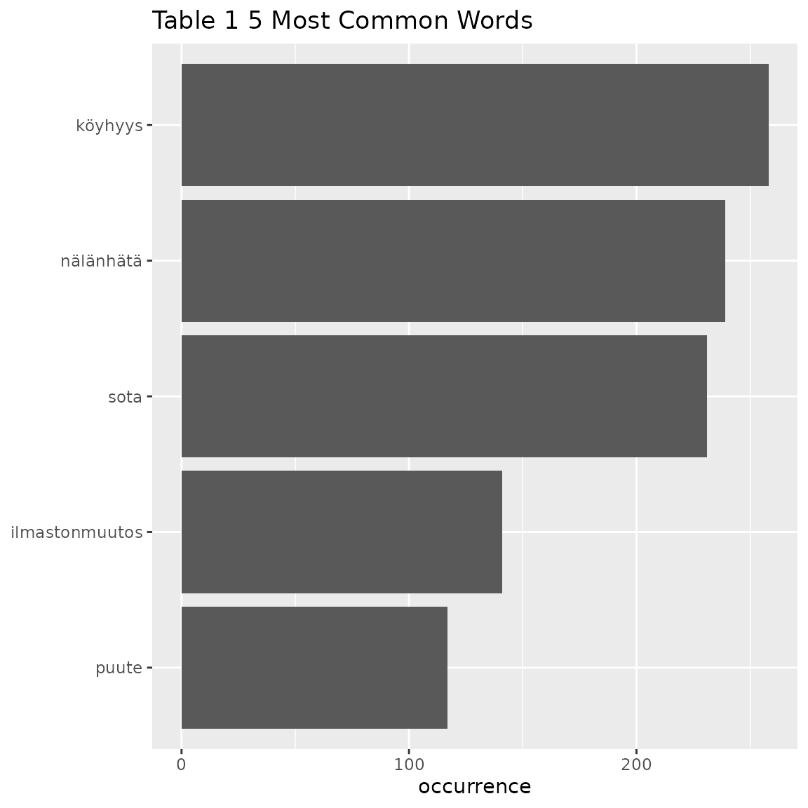

The arguments are:

table is the output of fst_get_top_words or fst_get_top_ngrams()
number The number of words/n-grams, default is 10.
name is an optional “name” for the plot, default is NULL

Make Top N-grams Tables functions

fst_ngrams_plot()

This functions plots the results of fst_get_top_ngrams().

fst_ngrams_plot(table = table3, number = 15, ngrams = 3, "Trigrams")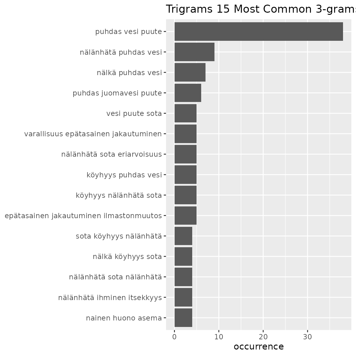

fst_ngrams_plot(table = table4, number = 15, ngrams = 2, "Bigrams")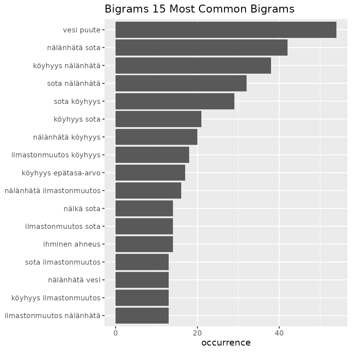

The arguments are:

table is the output of fst_get_top_words or fst_get_top_ngrams()
number The number of words/n-grams, default is 10.
name is an optional “name” for the plot, default is NULL
ngrams is the type of n-grams. As you can see above, you can plot top words using ngrams = 1.

Find and Plot Top Words function

fst_freq()

This functions runs fst_get_top_words() and fst_freq_plot() within one function:

fst_freq(data = df2, number = 12, strict = FALSE, name = "Q11_1")
#> Note:
#>  Words with equal occurrence are presented in alphabetical order. 
#>  With `strict` = FALSE, words occurring equally often as the `number` cutoff word will be displayed.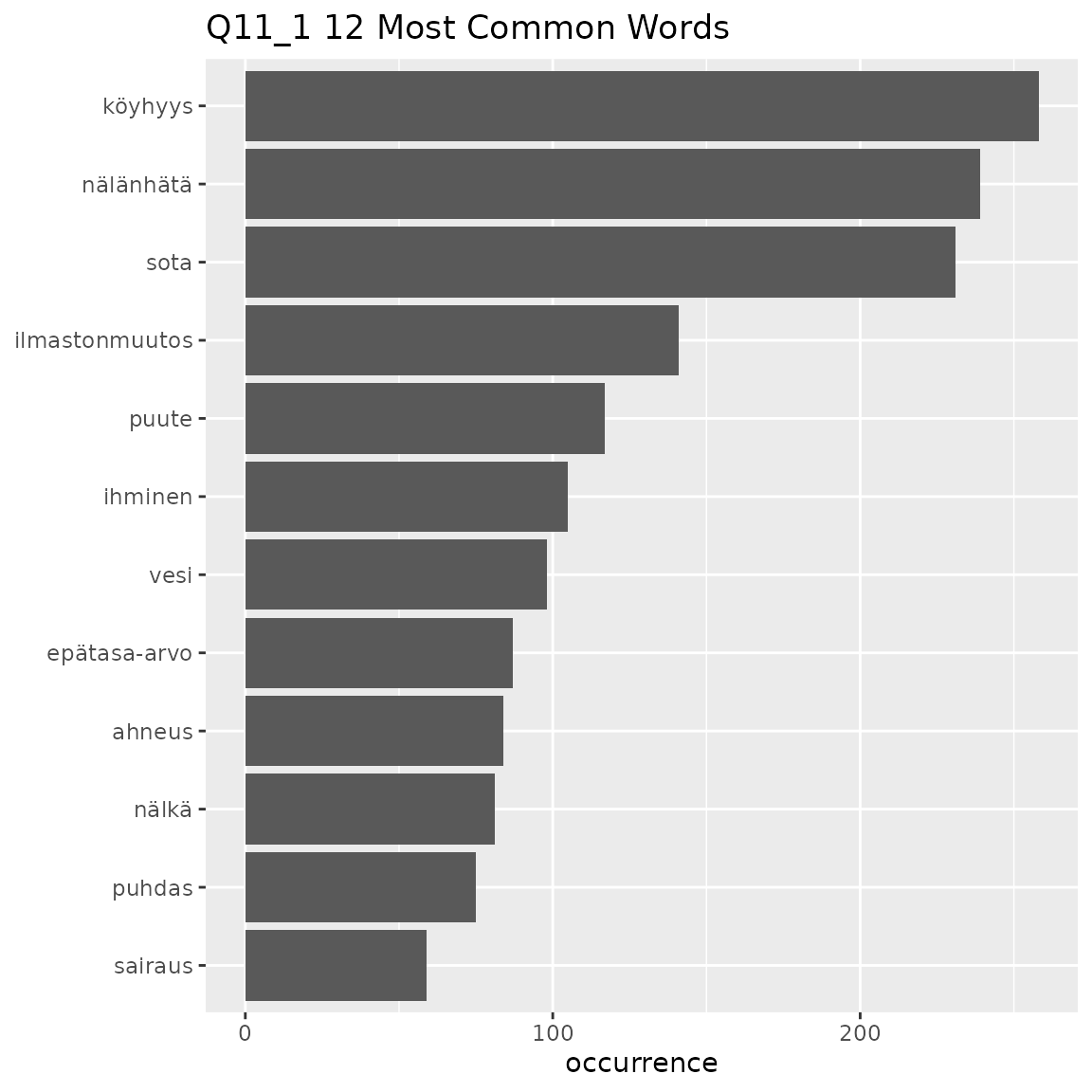

The arguments are as defined in the component functions:

data is output from data preparation, prepared data in CoNLL-U format, such as the output of fst_prepare_connlu().
number is the number of top words/n+grams to return, default is 10.
norm is the method for normalising the data. Valid settings are 'number_words' (the number of words in the responses, default), 'number_resp' (the number of responses), or NULL (raw count returned).
pos_filter is an optional list of which POS tags to include such as 'c("NOUN", "VERB", "ADJ", "ADV")'. The default is NULL, in which case all words in the data are considered.
strict is a boolean that determines how the function will deal with ‘ties’. If strict = TRUE, the table will cut-off at the exact number(words are presented in alphabetical order so later-alphabetically, equally occurring words to the word at number will not be shown.) If strict = FALSE, the table will show any words that occur equally frequently as the number cutoff word.
name is an optional “name” for the plot, default is NULL
use_svydesign_weights, svydesign, id and use_column_weights defined as above.

Find and Plot Top N-Grams function

fst_ngrams()

This functions runs fst_get_top_ngrams() and fst_ngrams_plot() within one function:

fst_ngrams(data = df1, number = 12, ngrams = 2)
#> Note:
#>  N-grams with equal occurrence are presented in alphabetical order. 
#>  By default, n-grams are presented in order to the `number` cutoff n-gram. 
#>  This means that equally-occurring later-alphabetically n-grams beyond the cutoff n-gram will not be displayed.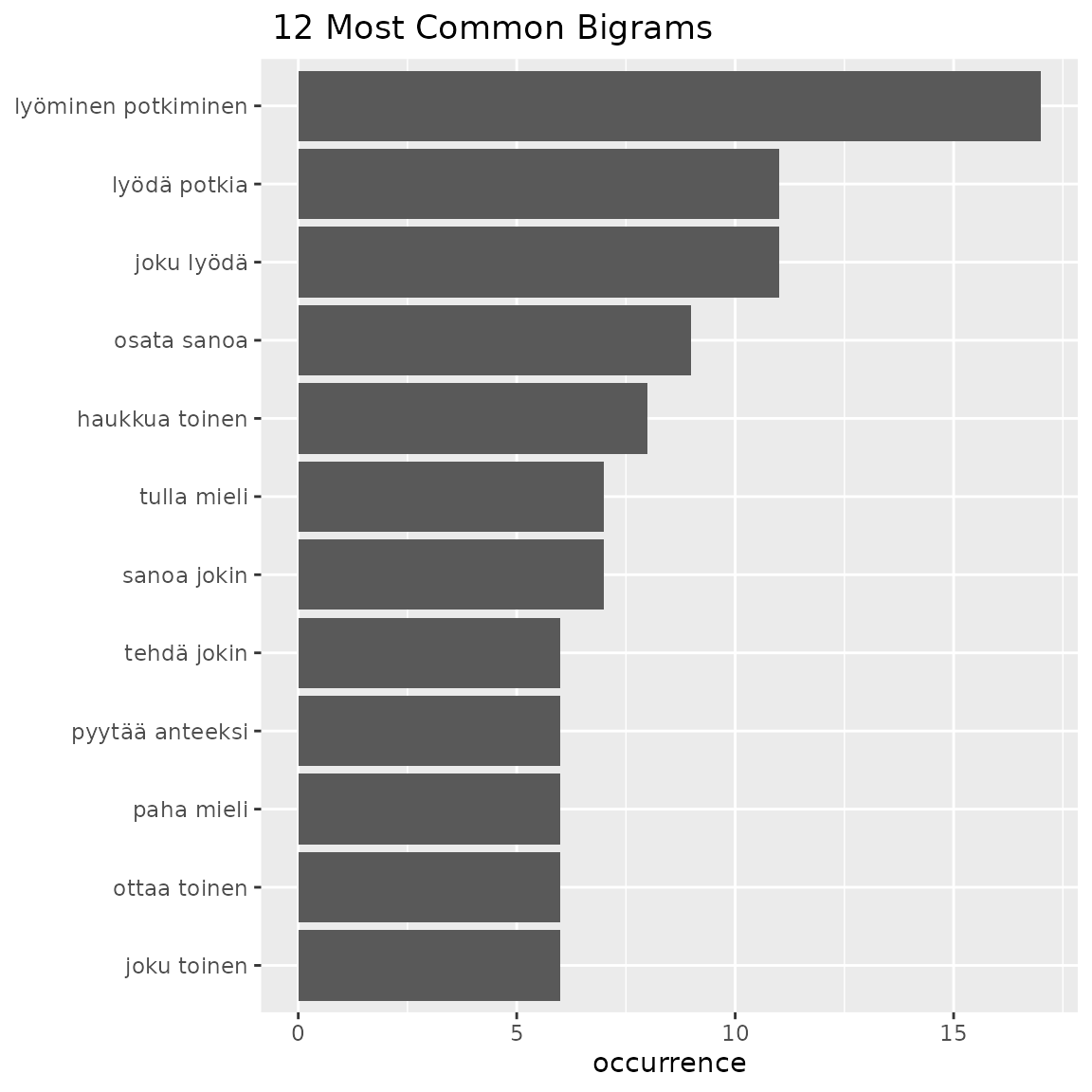

The arguments are as defined in the commponent functions:

data is output from data preparation, prepared data in CoNLL-U format, such as the output of fst_prepare_connlu().
number is the number of top words/n+grams to return, default is 10.
ngrams is the type of n-grams. The default is “1” (so top words). Set ngrams = 2 to get bigrams and n = 3 to get trigrams etc.
norm is the method for normalising the data. Valid settings are 'number_words' (the number of words in the responses, default), 'number_resp' (the number of responses), or NULL (raw count returned).
pos_filter is an optional list of which POS tags to include such as 'c("NOUN", "VERB", "ADJ", "ADV")'. The default is NULL, in which case all words in the data are considered.
strict is a boolean that determines how the function will deal with ‘ties’. If strict = TRUE, the table will cut-off at the exact number(n-grams are presented in alphabetical order so later-alphabetically, equally occurring n-grams to the n-gram at number will not be shown.) If strict = FALSE, the table will show any n-grams that occur equally frequently as the number cutoff word.
use_svydesign_weights, svydesign, id and use_column_weights defined as above.

Make Wordcloud function

fst_wordcloud()

This function will create a wordcloud plot for the data. There is an option to select only specific word types (POS tag).

fst_wordcloud(data = df1)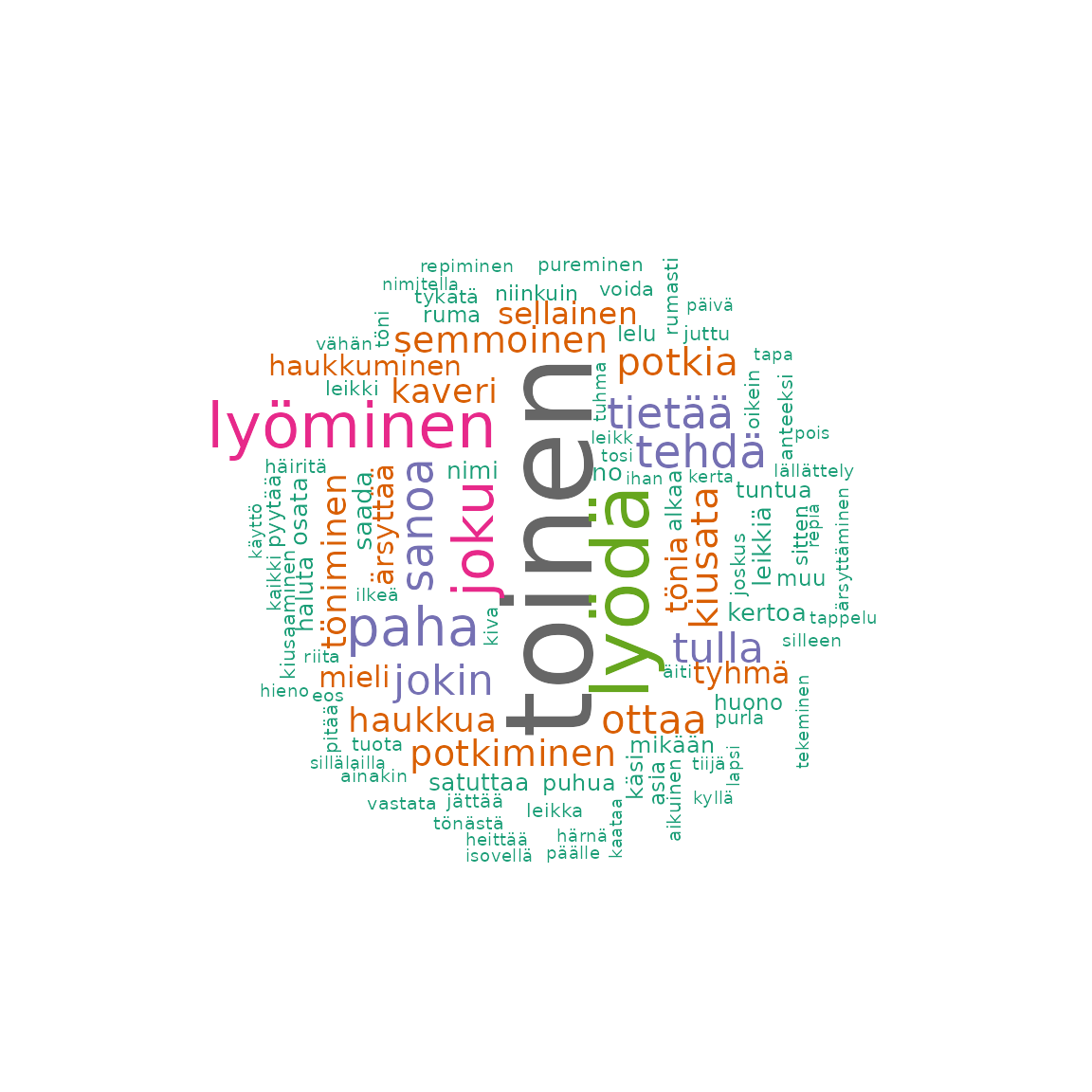

fst_wordcloud(
  data = df2,
  pos_filter = c("NOUN", "VERB", "ADJ", "ADV"),
  max = 150
)

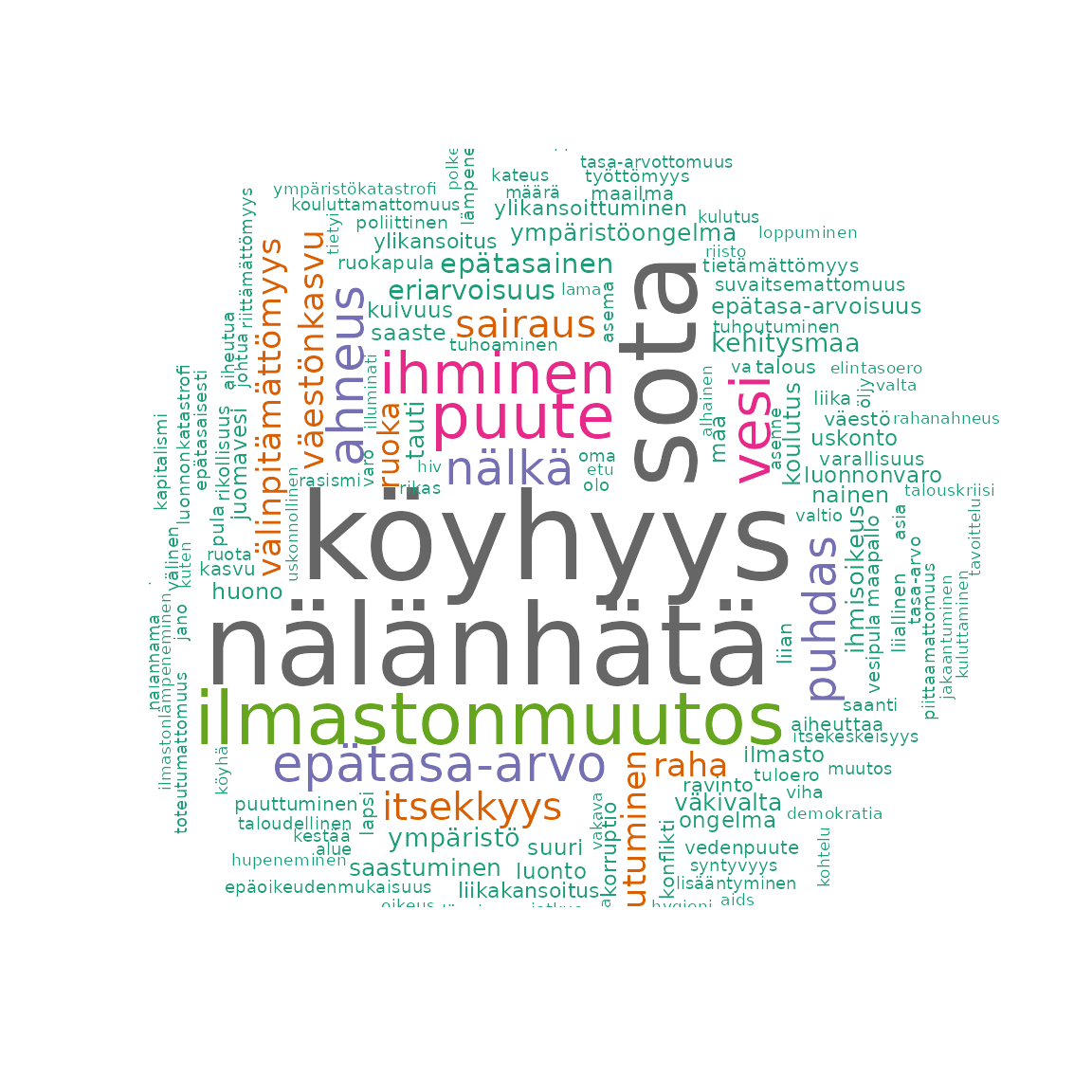
fst_wordclouds() takes 7 arguments:

data is output from data preparation, prepared data in CoNLL-U format, such as the output of fst_prepare_connlu().
pos_filter is an optional list of POS tags for inclusion in the wordcloud. The defaul is NULL.
max is the maximum number of words to display, the default is 100.
1. use_svydesign_weights, svydesign, id and use_column_weights defined as above.

Conclusion

EDA of open-ended survey questions can be conducted using functions in r/02_data_exploration.R such as finding most frequent words and n-grams, summarising the length of responses and words used, and visualising responses in word clouds. The results of this EDA can help researchers better understand their data, create hypotheses based on this initial insights, and inform future analysis of the surveys.

Citation

The Office of Ombudsman for Children: Child Barometer 2016 [dataset]. Version 1.0 (2016-12-09). Finnish Social Science Data Archive [distributor]. http://urn.fi/urn:nbn:fi:fsd:T-FSD3134

Finnish Children and Youth Foundation: Young People’s Views on Development Cooperation 2012 [dataset]. Version 2.0 (2019-01-22). Finnish Social Science Data Archive [distributor]. http://urn.fi/urn:nbn:fi:fsd:T-FSD2821