Overview-PackageTutorial • finnsurveytext

Overview of finnsurveytext

This tutorial aims to provide a simple overview of what is included within the finnsurveytext package and teach you how to use the main functions included in the package.

The below table shows you all the functions that are included in the package. The functions which are bolded are the main functions which are outlined in the sections below.

Section	Usage	Functions
1. Data Preparation	use the `udpipe` `R` package to clean and annotate the raw data into a standardised format (CoNLL-U) suitable for analysis.	fst_format() fst_format_svydesign() fst_print_available_models() fst_find_stopwords() fst_rm_stop_punct() fst_prepare() fst_prepare_svydesign()
2. Data Exploration	create wordclouds, n-gram tables and summary tables for initial insights into trends across responses.	fst_summarise_short() fst_summarise() fst_pos() fst_length_summary() fst_use_svydesign() fst_freq_table fst_ngrams_table() fst_ngrams_table2() fst_freq_plot() fst_ngrams_plot() fst_freq() fst_ngrams() fst_wordcloud()
3. Concept Network	creation of a concept network using the `textrank` `R` package with node size indicating word importance (PageRank) and edge weight showing co-occurrence of words.	fst_cn_search() fst_cn_edges() fst_cn_nodes() fst_cn_plot() fst_concept_network()
4. Comparison Functions	corresponding Data Exploration and Concept Network functions allowing for comparison between groups of survey respondents.	fst_pos_compare() fst_summarise_compare() fst_length_compare() fst_get_unique_ngrams_separate() fst_get_unique_ngrams() fst_join_unique() fst_ngrams_compare_plot() fst_freq_compare() fst_ngrams_compare() fst_comparison_cloud() fst_cn_get_unique_separate() fst_cn_get_unique() fst_cn_compare_plot() fst_concept_network_compare()
5. RShiny Demo App	A beta version of a UI for the package	runDemo()

0. Install and Load Package

First, the finnsurveytext package needs to be installed into your R environment and loaded into the environment. You may also want to load in the survey package if you want to use a svydesign object for the data and/or weights.

library(finnsurveytext)
library(survey)

1. Data Preparation

The data preparation functions are used to take your raw survey data (in a dataframe or svydesign object within your R environment) and convert it into a standardised format ready for analysis.

The functions in the remaining sections require your data to be pre-formatted into this format.

(To learn move about the format we use, see the Universal Dependencies Project.)

Option 1: Data is in a dataframe

The package comes with sample data. For this demonstration, we use dev_coop. The raw data looks like this:

fsd_id	q11_1	q11_2	q11_3	paino	gender	region	year_of_birth	education_level
1	elämiseen tarvittavat perusasiat ovat kehittymättöneet (esim. vesi, talo, ruoka). Ja niitä ei ole riittävästi	varmaan koitetaan kehittää em	saastuminen ja luonnonvarojen liikakäyttö, nälänhätä ja ylikansoittuminen	0.5440	Female	Etelä-Suomi	1992	NA
2	on kurjuutta ja nälänhätää, asiat eivät ole vielä kehittyneet, lapset eivät pääse kouluun, tytöillä on huonompi asema kuin pojilla.	pyritään auttamaan?	ihmiskauppa, nälänhätä ja sodat/turvattomuus	0.7171	Female	Pohjois- ja Itä-Suomi	1994	Matriculation examination
3	jokaisella ei ole turvattua toimeentuloa ja jossa todella huomaa koulutuksen arvon.	autetaan ja näytetään ihmisille tie parempaan tulevaisuuteen heidän oman työnsä tuloksena.	kouluttamattomuus, nälkä ja puhtaan veden puute.	0.6240	Female	Helsinki-Uusimaa	1994	Matriculation examination
4	kehityksen taso ei ole yhtä korkea kuin kehittyneissä maissa	yleensä haitataan kehitysmaan kehittymistä	öljy, raha, se fakta että ei olla vielä päästy asumaan muualla kuin tällä yhdellä planeetalla	0.3401	NA	Länsi-Suomi	NA	NA
5	asiat ovat vielä huonossa jamassa ja apua tarvitaan		eriarvoisuus, sodat, nälänhätä tietyissä maissa	0.6240	Female	Helsinki-Uusimaa	1993	Upper secondary vocational qualification

We will look at question 11_3 (responses to ‘’Jatka lausetta: Maailman kolme suurinta ongelmaa ovat… (Avokysymys)’) as our open-ended survey question. We also want to include our survey weights (in ‘paino’ column) and bring in the gender and region columns so we can use these values to compare groups.

The main function here is fst_prepare()

# FUNCTION DEFINITION
fst_prepare <- function(data,
                        question,
                        id,
                        model = "ftb",
                        stopword_list = "nltk",
                        language = "fi"
                        weights = NULL,
                        add_cols = NULL,
                        manual = FALSE,
                        manual_list = "")

We can run the function as follows:

df <- fst_prepare(data = dev_coop,
                  question = 'q11_3', 
                  id = 'fsd_id', 
                  weights = 'paino',
                  add_cols = c('gender', 'region')
                  )

Summary of components

data is the dataframe of interest. In this case, we are using data that comes with the package called “dev_coop”.
The question is the name of the column in your data which contains the open-ended survey question. In this example, we’re considering “q11_3”
id is the id column in our data, which is “fsd_id”
The function also requires a language model available for udpipe, in this case we are using the default Finnish Treebank, model = "ftb". (There are two options for Finnish language model; the other option is the Turku Dependency Treebank “tdt”.)
By default we will remove stopwords from the “nltk” stopword_list in this example. (To find the relevant lists of Finnish stopwords, you can run the fst_find_stopwords() function.) Punctuation is also removed from the data whenever stopwords are removed.
The default language is “fi”. This should be the two-letter ISO code for the language for the stopword list.
Optionally, you can add a weights column in your formatted data. Our weights are stored in the raw data as “paino”.
Optionally, you can add other columns to your formatted data (for use in comparison functions). We include our “gender” and “region” columns for this reason
The results in CoNLL-U format are stored in the local environment as df.
(manual and manual_list are used if you want to provide your own list of stopwords to remove from the data.)

The formatted data looks like this:

doc_id	paragraph_id	sentence_id	sentence	token_id	token	lemma	upos	xpos	feats	head_token_id	dep_rel	deps	misc	weight	gender	region
1	1	1	saastuminen ja luonnonvarojen liikakäyttö, nälänhätä ja ylikansoittuminen	1	saastuminen	saastuminen	NOUN	N,Sg,Nom	Case=Nom\|Number=Sing	0	root	NA	NA	0.544	Female	Etelä-Suomi
1	1	1	saastuminen ja luonnonvarojen liikakäyttö, nälänhätä ja ylikansoittuminen	3	luonnonvarojen	luonnonvaro	NOUN	N,Pl,Gen	Case=Gen\|Number=Plur	4	nmod	NA	NA	0.544	Female	Etelä-Suomi

Option 2: Data is in a svydesign object

The other option is to get your data from a svydesign object from the survey package. The survey package is a popular package used for analysing surveys.

The main function here is fst_prepare_svydesign()

# FUNCTION DEFINITION
fst_prepare_svydesign <- function(svydesign,
                                  question,
                                  id,
                                  model = "ftb",
                                  stopword_list = "nltk",
                                  language = "fi"
                                  use_weights = TRUE,
                                  add_cols = NULL,
                                  manual = FALSE,
                                  manual_list = "")

We can run the function as follows:

df2 <- fst_prepare_svydesign(svydesign = svy_dev,
                            question = 'q11_3', 
                            id = 'fsd_id', 
                            use_weights = TRUE,
                            add_cols = c('gender', 'region')
                            )

The only differences between the previous function and this one are:

svydesign is your svydesign object. In this case, we have one called “svy_dev”
The svydesign object has a component called “prob” which contains the inverse of the weights. Therefore, we use these by setting use_weights = TRUE

The formatted data looks like this (should look very similar to the above formatted data!):

doc_id	paragraph_id	sentence_id	sentence	token_id	token	lemma	upos	xpos	feats	head_token_id	dep_rel	deps	misc	weight	gender	region
1	1	1	saastuminen ja luonnonvarojen liikakäyttö, nälänhätä ja ylikansoittuminen	1	saastuminen	saastuminen	NOUN	N,Sg,Nom	Case=Nom\|Number=Sing	0	root	NA	NA	0.544	Female	Etelä-Suomi
1	1	1	saastuminen ja luonnonvarojen liikakäyttö, nälänhätä ja ylikansoittuminen	3	luonnonvarojen	luonnonvaro	NOUN	N,Pl,Gen	Case=Gen\|Number=Plur	4	nmod	NA	NA	0.544	Female	Etelä-Suomi

2. Data Exploration

Now that we have formatted data, we can begin data exploration. These functions are used to create summary tables and to find the most common themes in your survey responses.

Summary Tables

First, let’s create some summaries using fst_summarise, fst_pos and fst_length_summary

These functions are defined as follows:

# FUNCTION DEFINITIONS
fst_summarise <- function(data, 
                          desc = "All respondents") 

fst_pos <- function(data) 
  
fst_length_summary <- function(data,
                               desc = "All respondents",
                               incl_sentences = TRUE)

Summary of components

data is the formatted data.
desc is an optional name for the responses summarised, if not provided it will default to “All respondents”.
incl_sentences is an optional boolean for whether to also summarise sentence length (in addition to word length), if not provided it will default to TRUE.

Hence, these functions are run for our sample data as follows:

fst_summarise(df)

##     Description Respondents No Response Proportion Total Words Unique Words
## 1 All responses         945          25       0.97        4192         1132
##   Unique Lemmas
## 1           994

fst_pos(df)

##     UPOS                  UPOS_Name Count Proportion
## 1    ADJ                  adjective   389      0.093
## 2    ADP                 adposition    24      0.006
## 3    ADV                     adverb    64      0.015
## 4    AUX                  auxiliary     3      0.001
## 5  CCONJ   coordinating conjunction     3      0.001
## 6    DET                 determiner    28      0.007
## 7   INTJ               interjection     2      0.000
## 8   NOUN                       noun  3311      0.790
## 9    NUM                    numeral     5      0.001
## 10  PART                   particle    29      0.007
## 11  PRON                    pronoun    12      0.003
## 12 PROPN                proper noun    31      0.007
## 13 PUNCT                punctuation     0      0.000
## 14 SCONJ  subordinating conjunction     0      0.000
## 15   SYM                     symbol     1      0.000
## 16  VERB                       verb   278      0.066
## 17     X                      other    12      0.003

fst_length_summary(df)

## # A tibble: 2 × 8
##   Description              Respondents  Mean Minimum    Q1 Median    Q3 Maximum
##   <chr>                          <int> <dbl>   <int> <dbl>  <dbl> <dbl>   <int>
## 1 All responses- Words             920  5.52       1     4      5     6      32
## 2 All responses- Sentences         920  1.01       1     1      1     1       3

Identification of frequent words and phrases

Wordclouds

The first of our frequent words visualisations in the wordcloud which comes from the wordcloud package.

It is defined as follows:

# FUNCTION DEFINITION
fst_wordcloud <- function(data,
                          pos_filter = NULL,
                          max = 100,
                          use_svydesign_weights = FALSE,
                          id = "",
                          svydesign = NULL,
                          use_column_weights = FALSE)

Summary of components

data is the formatted data.
pos_filter is an optional list of POS tags for inclusion in the wordcloud. The default is NULL.
max is the maximum number of words to display, the default is 100.

Then, we have options for weighting the words in the cloud. These will all default to not include weights.

use_svydesign_weights should be set as TRUE if we want to use weights from within a svydesign object.
The id is only required if weights are coming from a svydesign object
The svydesign object

Here are some examples of creating wordclouds:

fst_wordcloud(df)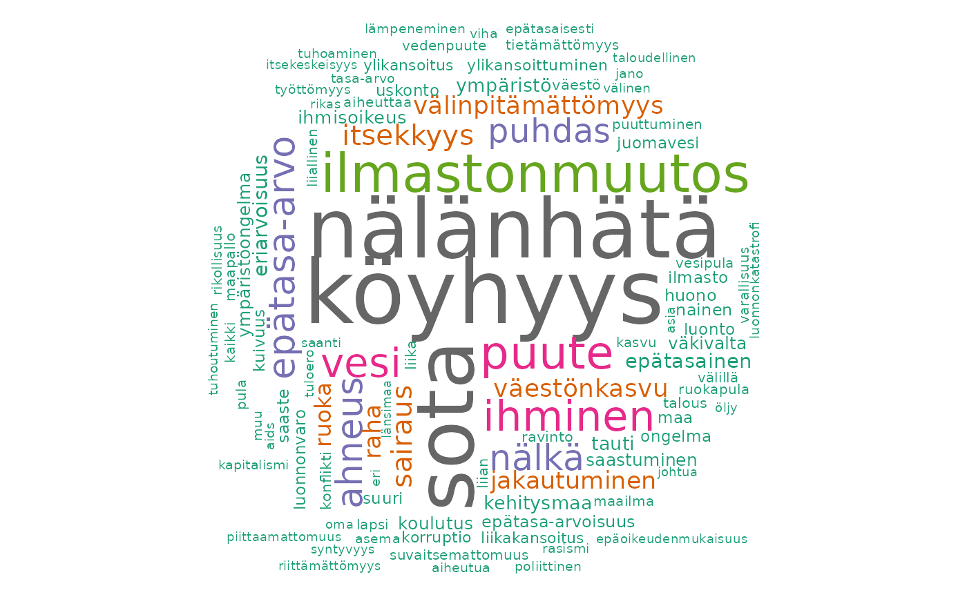

# We can only get weights from svydesign if they are NOT already in our formatted data. Hence we remove them for this demonstration!
df2$weight <- NULL
fst_wordcloud(df2, 
              pos_filter = c("NOUN", "VERB", "ADJ", "ADV"),
              max=100, 
              use_svydesign_weights = TRUE, 
              id = 'fsd_id', 
              svydesign = svy_dev)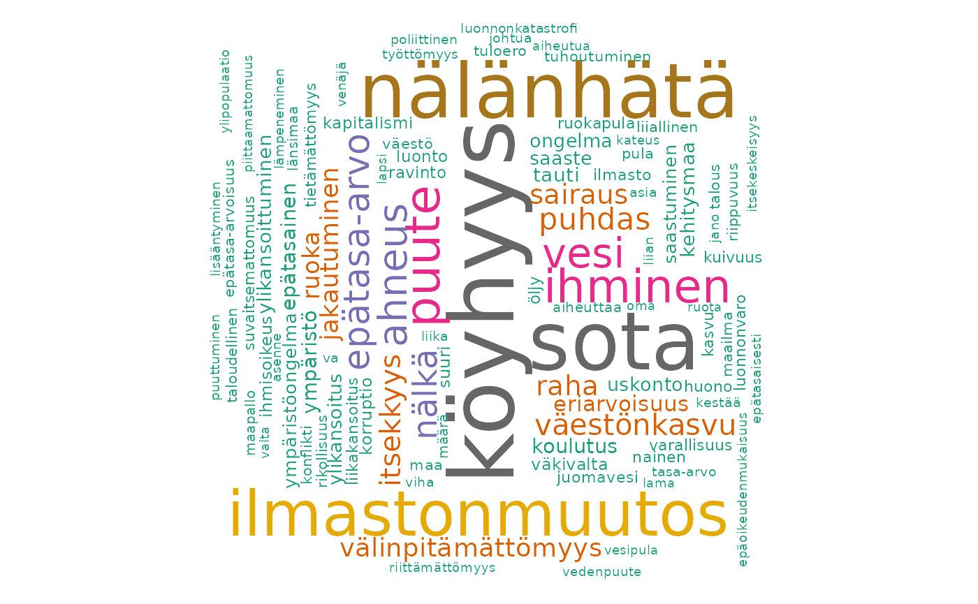

N-gram plots

Then, we have functions to identify and plot the most frequent words or n-grams (sets of n words in order).

# FUNCTION DEFINITIONS
fst_freq <- function(data,
                     number = 10,
                     norm = NULL,
                     pos_filter = NULL,
                     strict = TRUE,
                     name = NULL,
                     use_svydesign_weights = FALSE,
                     id = "",
                     svydesign = NULL,
                     use_column_weights = FALSE)
  
fst_ngrams <- function(data,
                       number = 10,
                       ngrams = 1,
                       norm = NULL,
                       pos_filter = NULL,
                       strict = TRUE,
                       name = NULL,
                       use_svydesign_weights = FALSE,
                       id = "",
                       svydesign = NULL,
                       use_column_weights = FALSE)

Summary of components

data is the formatted data.
number is the number of top words/ngrams to display
ngrams is the type of n-grams, default is 1.
norm is an optional method for normalising the data. Valid settings are “number_words” (the number of words in the responses), “number_resp” (the number of responses), or NULL (raw count returned, default, also used when weights are applied).
pos_filter is an optional list of POS tags for inclusion. The default is NULL.
strict is whether to strictly cut-off at number (ties are alphabetically ordered). The default value is TRUE.
The name is an optional “name” for the plot to add to title, default is NULL.

Then, we again have options for weighting the words in the plot. Again, these all default to not include weights.

use_svydesign_weights should be set as TRUE if we want to use weights from within a svydesign object.
The id is only required if weights are coming from a svydesign object
The svydesign object
use_svydesign_weights should be set as TRUE if we want to use weights from the weight column as set-up during the data formatting.

fst_freq(df)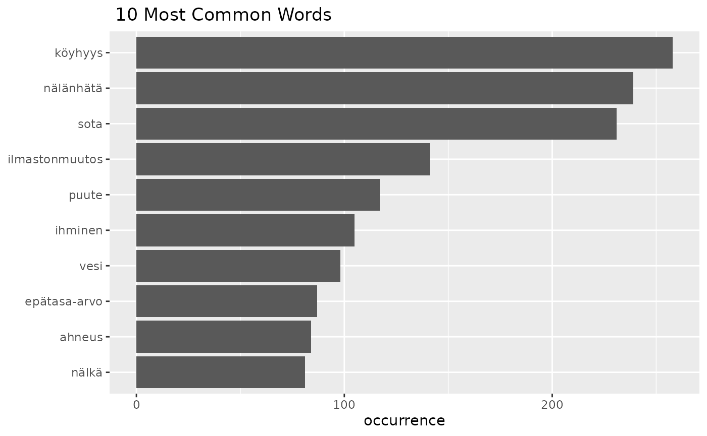

fst_ngrams(df, 
           number = 9, 
           ngrams = 2, 
           strict = FALSE,
           use_column_weights = TRUE)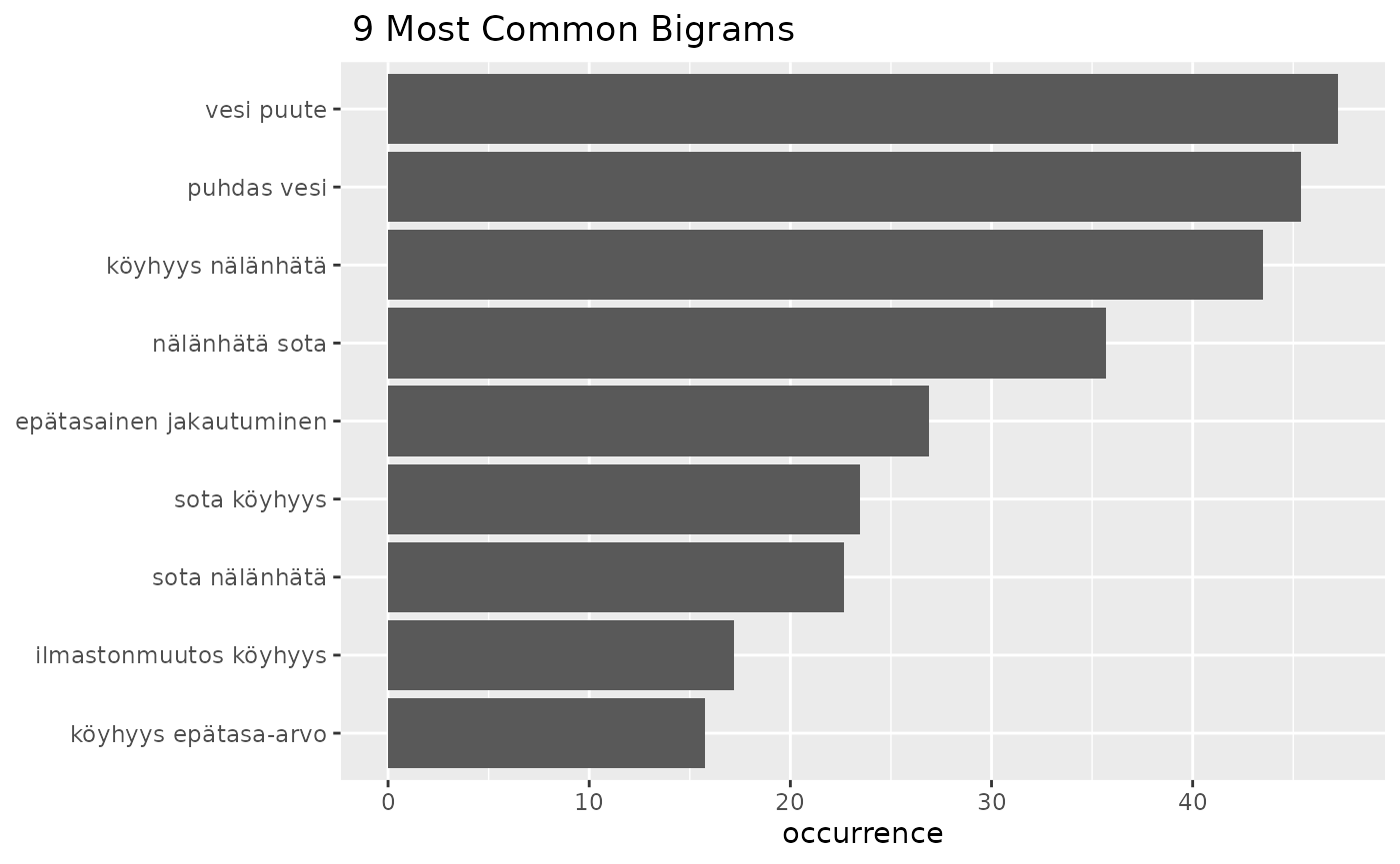

fst_freq(df,
         number = 5, 
         strict = FALSE,)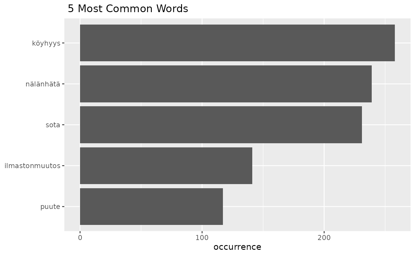

(fst_freq_table() and fst_ngrams_table() can be used to instead create tables of the top words.)

fst_freq_table(df, number = 15, strict = FALSE)

##                 words occurrence
## 1             köyhyys        258
## 2           nälänhätä        239
## 3                sota        231
## 4      ilmastonmuutos        141
## 5               puute        117
## 6             ihminen        105
## 7                vesi         98
## 8        epätasa-arvo         87
## 9              ahneus         84
## 10              nälkä         81
## 11             puhdas         75
## 12            sairaus         59
## 13          itsekkyys         58
## 14       väestönkasvu         48
## 15 välinpitämättömyys         47

3. Concept Network

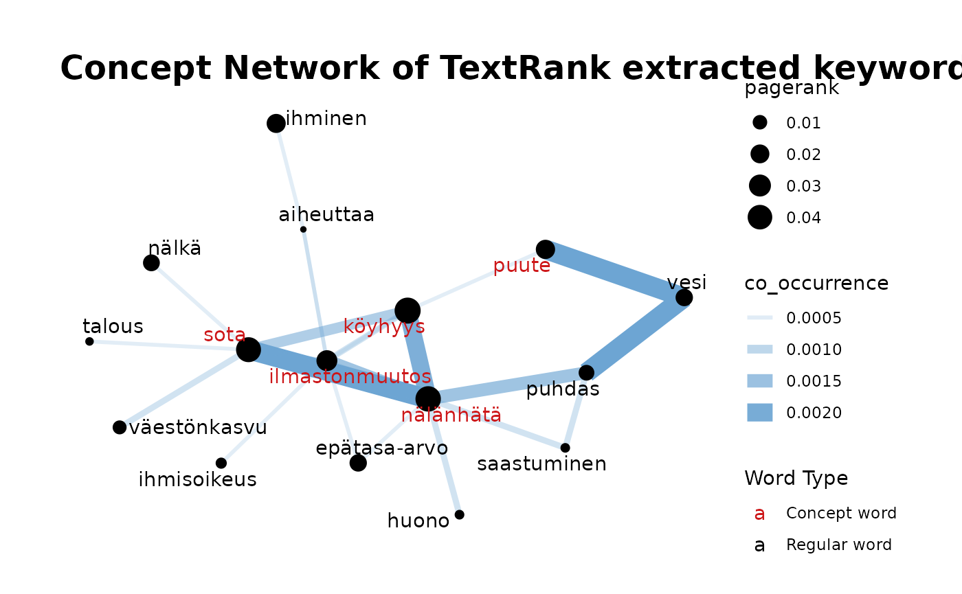
The finnsurveytext package currently contains our first iteration of a function which plots a concept network. These plots visualise keywords which are identified through the TextRank algorithm and maps co-occurrences between these terms. Vertices represent words with vertex size indicating word importance and co-occurrence between words is shown through edges with edge thickness indicating number of co-occurrences. Word importance is determined recursively (through the unsupervised TextRank algorithm, a graph-based ranking model for text processing) where words get more weight based on how many words co-occur and the weight of these co-occurring words. The concept network functions take search terms input by the user and the algorithm then suggests other words that are related to these input terms by co-occurrence. The input terms can be identified through functions in the package (such as fst_cn_search() or fst_freq_table()) or through other analysis separately conducted by the user. The concept network function can be used to identify concepts which could be individual words or a group of co-occurring words, or may contain a single ’concept’ whose component words are investigated and identified within a single network plot.

To utilise the TextRank algorithm in finnsurveytext, we use the textrank package. For further information on the package, please see this documentation. This package implements the TextRank and PageRank algorithms. (PageRank is the algorithm that Google uses to rank webpages.) You can read about the underlying TextRank algorithm here and about the PageRank algorithm here.

The main concept network function is fst_concept_network(). It is defined as follows:

# FUNCTION DEFINITIONS
fst_concept_network <- function(data,
                                concepts,
                                threshold = NULL,
                                norm = NULL,
                                pos_filter = NULL,
                                title = NULL)

Summary of components

data is the formatted data.
concepts are the concept words around which the network is created.
threshold is a minimum number of occurrences threshold for ‘edge’ between searched term and other word, default is NULL. Note, the threshold is applied before normalisation.
norm is an optional method for normalising the data. Valid settings are “number_words” (the number of words in the responses), “number_resp” (the number of responses), or NULL (raw count returned, default, also used when weights are applied).
pos_filter is an optional list of POS tags for inclusion. The default is NULL.
title is an optional title for plot, default is NULL and a generic title (“TextRank extracted keyword occurrences”) will be used.

For example, we can create the following concept network plots:

fst_concept_network(df, 
                    concepts = "köyhyys, nälänhätä, sota, ilmastonmuutos, puute", 
                    )

4. Comparison Functions

Recall that when we preprocessed the data, we included two additional columns, gender and region, to allow for comparison between respondents based on these values.

There are counterpart comparison functions for each of the functions we have shown above.

The comparison summary tables are defined as follows:

fst_pos_compare <- function(data,
                            field,
                            exclude_nulls = FALSE,
                            rename_nulls = 'null_data')

fst_summarise_compare <- function(data,
                                  field,
                                  exclude_nulls = FALSE,
                                  rename_nulls = 'null_data')

fst_length_compare <- function(data,
                               field,
                               incl_sentences = TRUE,
                               exclude_nulls = FALSE,
                               rename_nulls = 'null_data')

Summary of Components

data is the formatted data.
field is the column in data used for splitting groups
We can choose whether to include or exclude surveys with no response in our splitting column by setting exclude_nulls. The default value is FALSE.
rename_nulls is what to fill empty values with if exclude_nulls = FALSE.

Let’s compare our responses based on the region of the respondent:

knitr::kable(fst_pos_compare(df, 'region'))

UPOS	Part_of_Speech_Name	Etelä-Suomi-Count	Etelä-Suomi-Prop	Helsinki-Uusimaa-Count	Helsinki-Uusimaa-Prop	Länsi-Suomi-Count	Länsi-Suomi-Prop	Pohjois- ja Itä-Suomi-Count	Pohjois- ja Itä-Suomi-Prop	null_data-Count	null_data-Prop
ADJ	adjective	79	0.101	118	0.098	105	0.082	84	0.093	3	0.188
ADP	adposition	4	0.005	11	0.009	6	0.005	3	0.003	0	0.000
ADV	adverb	8	0.010	20	0.017	22	0.017	13	0.014	1	0.062
AUX	auxiliary	1	0.001	1	0.001	1	0.001	0	0.000	0	0.000
CCONJ	coordinating conjunction	1	0.001	0	0.000	1	0.001	1	0.001	0	0.000
DET	determiner	6	0.008	10	0.008	7	0.005	5	0.006	0	0.000
INTJ	interjection	0	0.000	2	0.002	0	0.000	0	0.000	0	0.000
NOUN	noun	610	0.776	936	0.774	1028	0.805	725	0.802	12	0.750
NUM	numeral	1	0.001	1	0.001	3	0.002	0	0.000	0	0.000
PART	particle	2	0.003	15	0.012	9	0.007	3	0.003	0	0.000
PRON	pronoun	1	0.001	4	0.003	3	0.002	4	0.004	0	0.000
PROPN	proper noun	3	0.004	12	0.010	14	0.011	2	0.002	0	0.000
PUNCT	punctuation	0	0.000	0	0.000	0	0.000	0	0.000	0	0.000
SCONJ	subordinating conjunction	0	0.000	0	0.000	0	0.000	0	0.000	0	0.000
SYM	symbol	0	0.000	1	0.001	0	0.000	0	0.000	0	0.000
VERB	verb	69	0.088	72	0.060	75	0.059	62	0.069	0	0.000
X	other	1	0.001	6	0.005	3	0.002	2	0.002	0	0.000

knitr::kable(fst_summarise_compare(df, 'region'))

Description	Respondents	No Response	Proportion	Total Words	Unique Words	Unique Lemmas
Etelä-Suomi	176	0	1.00	786	360	336
Helsinki-Uusimaa	269	10	0.96	1209	493	443
Länsi-Suomi	284	8	0.97	1277	478	425
Pohjois- ja Itä-Suomi	213	7	0.97	904	338	309
null_data	3	0	1.00	16	16	16

knitr::kable(fst_length_compare(df, 'region'))

Description	Respondents	Mean	Minimum	Q1	Median	Q3	Maximum
Etelä-Suomi- Words	176	5.483	2	4.0	5	6	23
Etelä-Suomi- Sentences	176	1.017	1	1.0	1	1	3
Helsinki-Uusimaa- Words	259	5.579	1	4.0	5	6	25
Helsinki-Uusimaa- Sentences	259	1.023	1	1.0	1	1	3
Länsi-Suomi- Words	276	5.620	1	4.0	5	6	32
Länsi-Suomi- Sentences	276	1.007	1	1.0	1	1	2
Pohjois- ja Itä-Suomi- Words	206	5.311	1	4.0	5	6	20
Pohjois- ja Itä-Suomi- Sentences	206	1.015	1	1.0	1	1	2
null_data- Words	3	6.333	5	5.5	6	7	8
null_data- Sentences	3	1.000	1	1.0	1	1	1

The ngrams comparison functions are defined similarly (with some additional new values):

# FUNCTION DEFINITIONS
fst_freq_compare <- function(data,
                             field,
                             number = 10,
                             norm = NULL,
                             pos_filter = NULL,
                             strict = TRUE,
                             use_svydesign_weights = FALSE,
                             id = "",
                             svydesign = NULL,
                             use_column_weights = FALSE,
                             exclude_nulls = FALSE,
                             rename_nulls = 'null_data',
                             unique_colour = "indianred",
                             title_size = 20,
                             subtitle_size = 15)


fst_ngrams_compare <- function(data,
                              field,
                              number = 10,
                              ngrams = 1,
                              norm = NULL,
                              pos_filter = NULL,
                              strict = TRUE,
                              use_svydesign_weights = FALSE,
                              id = "",
                              svydesign = NULL,
                              use_column_weights = FALSE,
                              exclude_nulls = FALSE,
                              rename_nulls = 'null_data',
                              unique_colour = "indianred",
                              title_size = 20,
                              subtitle_size = 15)

The new components are:

unique_colour is chosen to differentiate values which are unique to one group of respondents, the default is “indianred”
title_size and subtitle_size set these, you may need to change them from the default values if any of your group names are long or if there are many groups.

For the ngrams, let’s compare respondents by gender.

fst_freq_compare(df, 
                 'gender', 
                 use_column_weights = TRUE,
                 exclude_nulls = TRUE)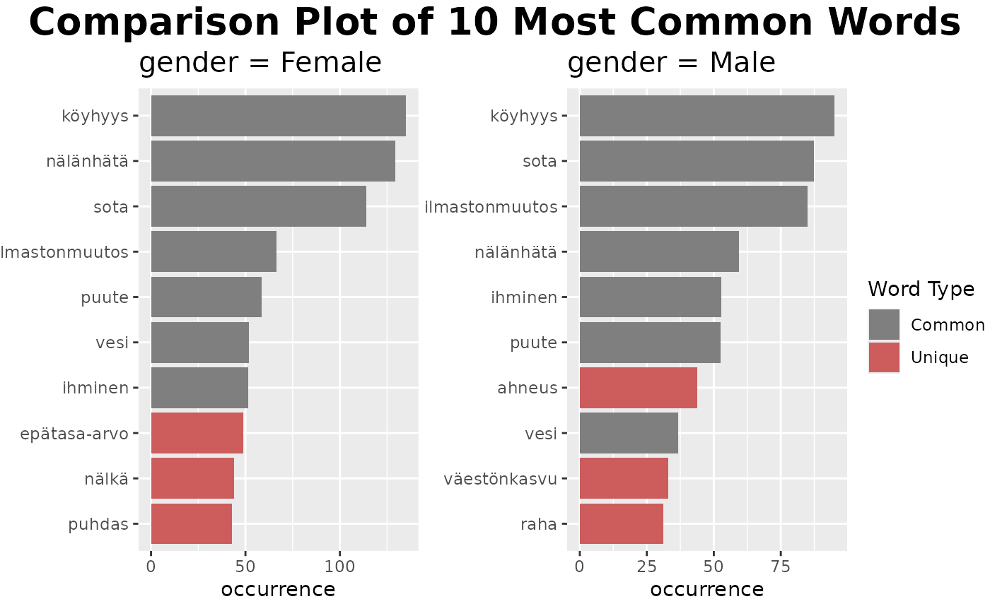

fst_ngrams_compare(df, 
                   'gender', 
                   ngrams = 2, 
                   use_column_weights = TRUE, 
                   exclude_nulls = TRUE)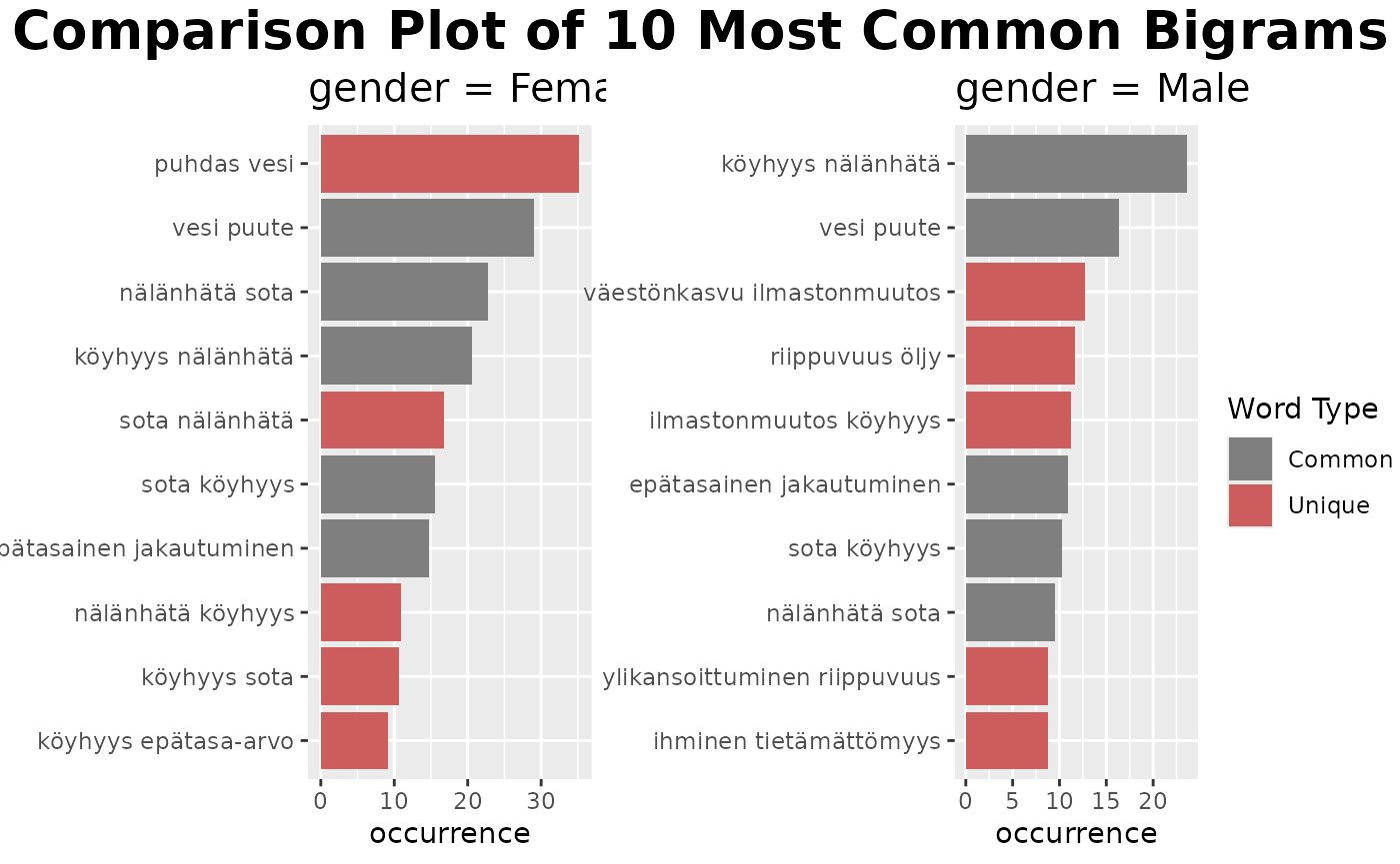

The comparison cloud extends the wordcloud concept.

A comparison cloud compares the relative frequency with which a term is used in two or more documents. This cloud shows words that occur more regularly in responses from a specific type of respondent. For more information about comparison clouds, you can read this documentation.

The comparison cloud is defined as follows, with settings as defined for the previous functions:

# FUNCTION DEFINITION
fst_comparison_cloud <- function(data,
                                 field,
                                 pos_filter = NULL,
                                 norm = NULL,
                                 max = 100,
                                 use_svydesign_weights = FALSE,
                                 id = "",
                                 svydesign = NULL,
                                 use_column_weights = FALSE,
                                 exclude_nulls = FALSE,
                                 rename_nulls = "null_data")

Thus, we can create comparison clouds:

fst_comparison_cloud(df, 'gender', max = 40, use_column_weights = TRUE, exclude_nulls = TRUE)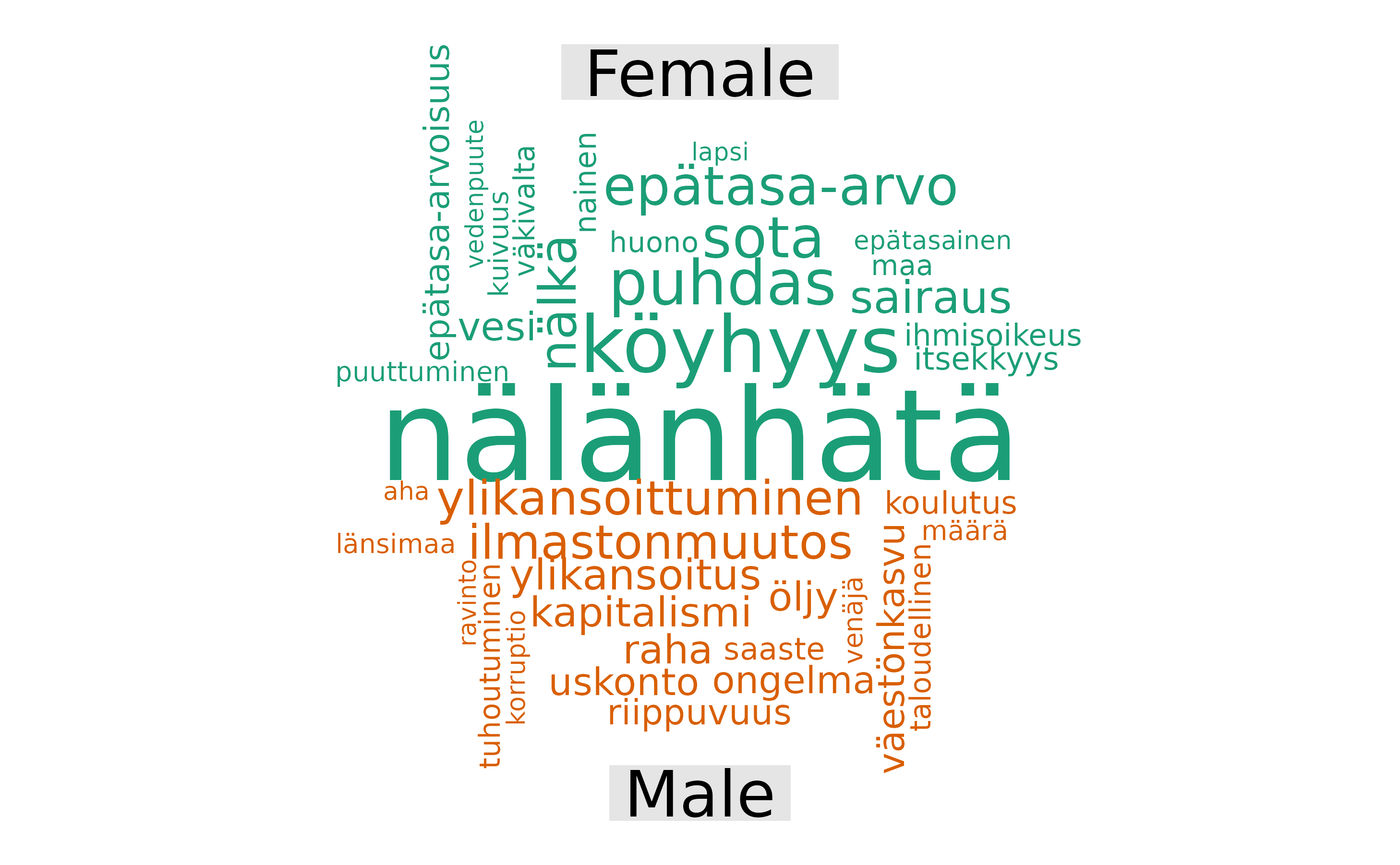

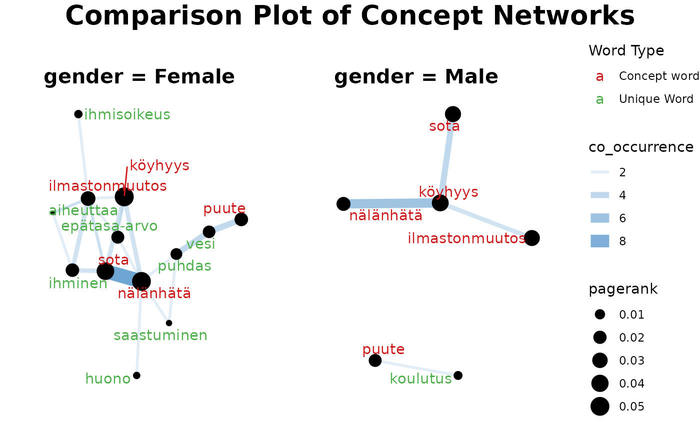
Finally we have the comparison concept network which has the following components which should be familiar from previous functions:

# FUNCTION DEFINITION
fst_concept_network_compare <- function(data,
                                        concepts,
                                        field,
                                        norm = NULL,
                                        threshold = NULL,
                                        pos_filter = NULL,
                                        exclude_nulls = FALSE,
                                        rename_nulls = 'null_data',
                                        title_size = 20,
                                        subtitle_size = 15)

We run the comparison concept network as follows:

fst_concept_network_compare(df, 
                            concepts = "köyhyys, nälänhätä, sota, ilmastonmuutos, puute", 
                            'gender',
                            exclude_nulls = TRUE
                            )

For more information on the finnsurveytext functions, see the package website and documentation available from the CRAN.

Data

The package comes with sample data from two Finnish surveys obtained from the Finnish Social Science Data Archive an a survey in English available from GESIS:

1. Child Barometer Data

Source: FSD3134 Lapsibarometri 2016
Question: q7 ‘Kertoisitko, mitä sinun mielestäsi kiusaaminen on? (Avokysymys)’
Licence: (A) openly available for all users without registration (CC BY 4.0).
Link to Data: https://urn.fi/urn:nbn:fi:fsd:T-FSD3134

2. Development Cooperation Data

Source: FSD2821 Nuorten ajatuksia kehitysyhteistyöstä 2012
Questions: q11_1 ‘Jatka lausetta: Kehitysmaa on maa, jossa… (Avokysymys)’, q11_2 ‘Jatka lausetta: Kehitysyhteistyö on toimintaa, jossa… (Avokysymys)’, q11_3 ‘Jatka lausetta: Maailman kolme suurinta ongelmaa ovat… (Avokysymys)’
Licence: (A) openly available for all users without registration (CC BY 4.0).
Link to Data: https://urn.fi/urn:nbn:fi:fsd:T-FSD2821

3. Patient Joe (open-ended question)

Source: GESIS – Leibniz Institute for the Social Sciences
Open-ended question: ‘Joe’s doctor told him that he would need to return in two weeks to find out whether or not his condition had improved. But when Joe asked the receptionist for an appointment, he was told that it would be over a month before the next available appointment. What should Joe do?’
Licence: CC BY 4.0: Attribution
Link to Data: https://doi.org/10.7802/2474