Tutorial6-Example_of_analysis_of_an_open-ended_survey

Introduction

This tutorial demonstrates the use of the package to analyse a survey question. It is intended to demonstrate the use of the package from start to finish in detail. In this example, we look at responses split by gender but it is expected that you might look at a variety of different splits of your data in analysis.

Installation of package.

Once the package is installed, you can load the finnsurveytext package as below: (Other required packages such as dplyr and stringr will also be installed if they are not currently installed in your environment.)

library(finnsurveytext)

The Question

We will look at our Q11_3 data from the Development Cooperation 2012 survey data which is included as sample data with our package. The specific question we’re looking at is as follows:

q11_3 Jatka lausetta: Maailman kolme suurinta ongelmaa ovat… (Avokysymys)
- q11_3 Continue the sentence: The world’s three biggest problems are… (Open question)

Overview of Functions

This tutorial covers functions from throughout the package. For further details on the functions, see the previous tutorials.

The Data

There are four sets of data files available within the package which are used in this tutorial

Development Cooperation Data Split by Gender

data/dev_data.rda - All responses to the survey
data/dev_data_m.rda - Responses to the survey by participants who have listed their gender as male
data/dev_data_f.rda - Responses to the survey by participants who have listed their gender as female
data/dev_data_na.rda - Responses to the survey by participants who have not responded to the gender question

Below, we prepare the data. (For further explanation of these functions, see Tutorial1-Prepare CoNLL-U.)

all <- fst_prepare_conllu(
  data = dev_data,
  field = "q11_3",
  stopword_list = "none"
)

all_nltk <- fst_prepare_conllu(
  data = dev_data,
  field = "q11_3",
  stopword_list = "nltk"
)

female <- fst_prepare_conllu(
  data = dev_data_f,
  field = "q11_3",
  stopword_list = "none"
)

female_nltk <- fst_prepare_conllu(
  data = dev_data_f,
  field = "q11_3",
  stopword_list = "nltk"
)

male <- fst_prepare_conllu(
  data = dev_data_m,
  field = "q11_3",
  stopword_list = "none"
)

male_nltk <- fst_prepare_conllu(
  data = dev_data_m,
  field = "q11_3",
  stopword_list = "nltk"
)

na <- fst_prepare_conllu(
  data = dev_data_na,
  field = "q11_3",
  stopword_list = "none"
)

na_nltk <- fst_prepare_conllu(
  data = dev_data_na,
  field = "q11_3",
  stopword_list = "nltk"
)

The following is an excerpt from one of our prepared datasets:

knitr::kable(head(all_nltk, 10))

doc_id	paragraph_id	sentence_id	sentence	token_id	token	lemma	upos	xpos	feats	head_token_id	dep_rel	deps	misc
doc1	1	1	saastuminen ja luonnonvarojen liikakäyttö, nälänhätä ja ylikansoittuminen	1	saastuminen	saastuminen	NOUN	N,Sg,Nom	Case=Nom\|Number=Sing	0	root	NA	NA
doc1	1	1	saastuminen ja luonnonvarojen liikakäyttö, nälänhätä ja ylikansoittuminen	3	luonnonvarojen	luonnonvaro	NOUN	N,Pl,Gen	Case=Gen\|Number=Plur	4	nmod	NA	NA
doc1	1	1	saastuminen ja luonnonvarojen liikakäyttö, nälänhätä ja ylikansoittuminen	4	liikakäyttö	liikakäyttö	NOUN	N,Sg,Nom	Case=Nom\|Number=Sing	1	conj	NA	SpaceAfter=No
doc1	1	1	saastuminen ja luonnonvarojen liikakäyttö, nälänhätä ja ylikansoittuminen	6	nälänhätä	nälänhätä	NOUN	N,Sg,Nom	Case=Nom\|Number=Sing	1	conj	NA	NA
doc1	1	1	saastuminen ja luonnonvarojen liikakäyttö, nälänhätä ja ylikansoittuminen	8	ylikansoittuminen	ylikansoittuminen	NOUN	N,Sg,Nom	Case=Nom\|Number=Sing	1	conj	NA	SpacesAfter=
doc2	1	1	ihmiskauppa, nälänhätä ja sodat/turvattomuus	1	ihmiskauppa	ihmiskauppa	NOUN	N,Sg,Nom	Case=Nom\|Number=Sing	0	root	NA	SpaceAfter=No
doc2	1	1	ihmiskauppa, nälänhätä ja sodat/turvattomuus	3	nälänhätä	nälänhätä	NOUN	N,Sg,Nom	Case=Nom\|Number=Sing	1	conj	NA	NA
doc2	1	1	ihmiskauppa, nälänhätä ja sodat/turvattomuus	5	sodat/turvattomuus	sodat/turvattomuus	NOUN	N,Sg,Nom	Case=Nom\|Number=Sing	1	conj	NA	SpacesAfter=
doc3	1	1	kouluttamattomuus, nälkä ja puhtaan veden puute.	1	kouluttamattomuus	kouluttamattomuus	NOUN	N,Sg,Nom	Case=Nom\|Number=Sing	0	root	NA	SpaceAfter=No
doc3	1	1	kouluttamattomuus, nälkä ja puhtaan veden puute.	3	nälkä	nälkä	NOUN	N,Sg,Nom	Case=Nom\|Number=Sing	1	conj	NA	NA

Analysis

First, let’s consider all the data to get some initial information about the responses to this question. We will run the following functions:

For further information on these functions, please see “Tutorial2-Data_exploration”.

knitr::kable(
  fst_summarise(all_nltk)
)

Description	Respondents	No Response	Proportion	Total Words	Unique Words	Unique Lemmas
All respondents	945	25	0.97	4192	1132	994


knitr::kable(
  fst_pos(all_nltk)
)

UPOS	UPOS_Name	Count	Proportion
ADJ	adjective	389	0.093
ADP	adposition	24	0.006
ADV	adverb	64	0.015
AUX	auxiliary	3	0.001
CCONJ	coordinating conjunction	3	0.001
DET	determiner	28	0.007
INTJ	interjection	2	0.000
NOUN	noun	3311	0.790
NUM	numeral	5	0.001
PART	particle	29	0.007
PRON	pronoun	12	0.003
PROPN	proper noun	31	0.007
SYM	symbol	1	0.000
VERB	verb	278	0.066
X	other	12	0.003


knitr::kable(
  fst_length_summary(all_nltk)
)

Description	Respondents	Mean	Minimum	Q1	Median	Q3	Maximum
All respondents- Words	920	5.515217	1	4	5	6	32
All respondents- Sentences	920	1.015217	1	1	1	1	3

Remarks:

We have an overall response rate of 97%. We might wonder, is this response rate consist across different types of survey participants?
Responses consist mostly of adjectives (10% of words in stopwords-removed responses), nouns (80%) and verbs (7%)
Responses to this question are between 1 and 32 words, and between 1 and 3 sentences. Most responses seem to be 1 sentence with an average of 4-5 words.

fst_wordcloud(all_nltk)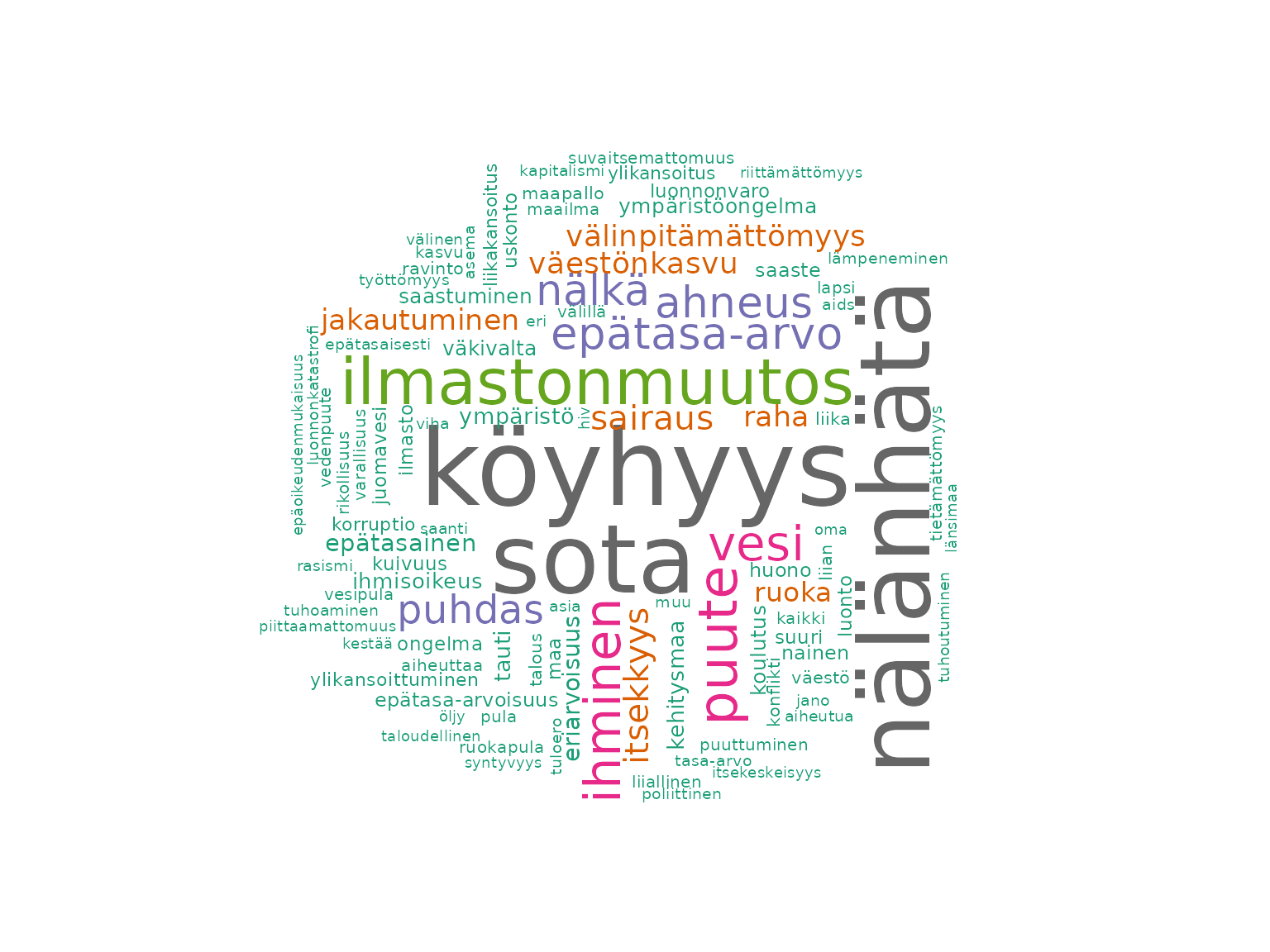

Remarks:

Top words seem to be ‘nälänhätä’, ‘köyhyys’, ‘sota’
Next tier of common words might be: ‘vesi’ ‘puute’, ‘ihminen’, ‘ilmastonmuutos’, ‘ahneus’, ‘nälka’, ‘epätasa-arvo’

Translations

‘köyhyys’ = poverty
‘nälänhätä’ = famine
‘sota’ = war
‘vesi’ = water
‘puute’ = lack of
‘ihminen’ = human
‘ilmastonmuutos’ = climate change
‘ahneus’ = greed
‘nälka’ = hunger
‘epätasa-arvo’ = inequality

Top N-Grams

Next, we will look at the most common words (unigrams), bigrams and trigrams in that data.

fst_freq(all_nltk, 10, strict = FALSE, norm = "number_resp")
#> Note:
#>  Words with equal occurrence are presented in alphabetical order. 
#>  With `strict` = FALSE, words occurring equally often as the `number` cutoff word will be displayed.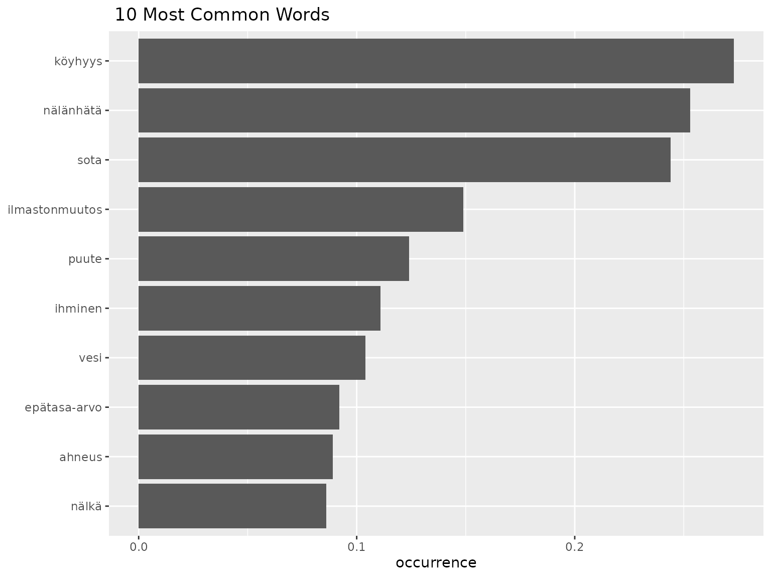

fst_ngrams(all_nltk, 10, ngrams = 2, strict = FALSE, norm = "number_resp")
#> Note:
#>  N-grams with equal occurrence are presented in alphabetical order. 
#>  With `strict` = FALSE, n-grams occurring equally often as the `number` cutoff n-gram will be displayed.

knitr::kable(
  fst_get_top_ngrams(all_nltk,
                              number = 10,
                              ngrams = 2,
                              norm = "number_words",
                              pos_filter = NULL,
                              strict = FALSE)
)
#> Note:
#>  N-grams with equal occurrence are presented in alphabetical order. 
#>  With `strict` = FALSE, n-grams occurring equally often as the `number` cutoff n-gram will be displayed.

words	occurrence
puhdas vesi	0.015
vesi puute	0.013
nälänhätä sota	0.010
köyhyys nälänhätä	0.009
sota nälänhätä	0.008
epätasainen jakautuminen	0.007
sota köyhyys	0.007
köyhyys sota	0.005
nälänhätä köyhyys	0.005
köyhyys epätasa-arvo	0.004
ilmastonmuutos köyhyys	0.004
nälänhätä ilmastonmuutos	0.004

fst_ngrams(all_nltk, 10, ngrams = 3, strict = FALSE, norm = "number_resp")
#> Note:
#>  N-grams with equal occurrence are presented in alphabetical order. 
#>  With `strict` = FALSE, n-grams occurring equally often as the `number` cutoff n-gram will be displayed.

Remarks:

Note here that we have set norm = 'number_resp' as we’re interested in the proportion of responses that list as specific word.
- Leaving norm = 'number_words (the default) would still be comparible between the genders, but in this case the norm we’ve chosen is more interpretable (and we don’t expect many words to be repeated in responses).
We see the top words we identified previously
- Around 1/4 of respondents list each of ‘nälänhätä’, ‘köyhyys’, ‘sota’
We get more context on ‘vesi’ here in the bigrams. This makes sense since ‘water’ alone doesn’t describe a common international ‘problem’.
- ‘puhdas vesi’ = clean water
- ‘vesi puute’ = lack of water
- ‘puhdas vesi puute’ is the most common trigram.
We can assume that answers like ‘nälänhätä sota’ are probably from listing different terms in responses. So, some bigrams are more meaningful than others.

A Concept Network

Next, let’s look at some Concept Networks before we look into gender. (For further detail on the Concept Network functions, see “Tutorial3-Overview_of_Concept_Network_functions”.) Our Concept Network function can be used to visualise the words that occur around our words of interest.

Again, we will set norm = 'number_resp'.

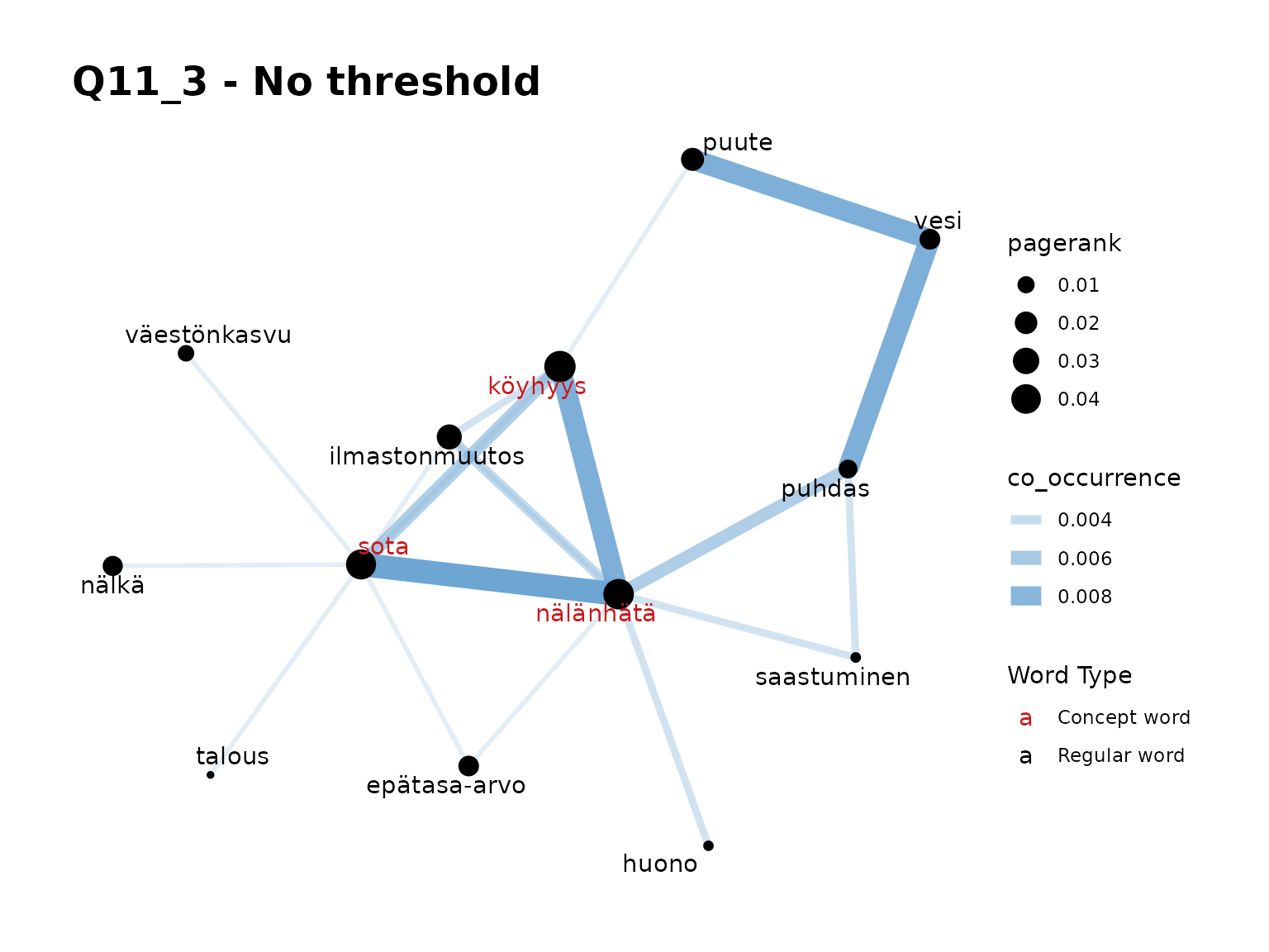
fst_concept_network(all_nltk,
  concepts = "köyhyys, nälänhätä, sota",
  title = "Q11_3 - No threshold",
  norm = "number_resp"
)

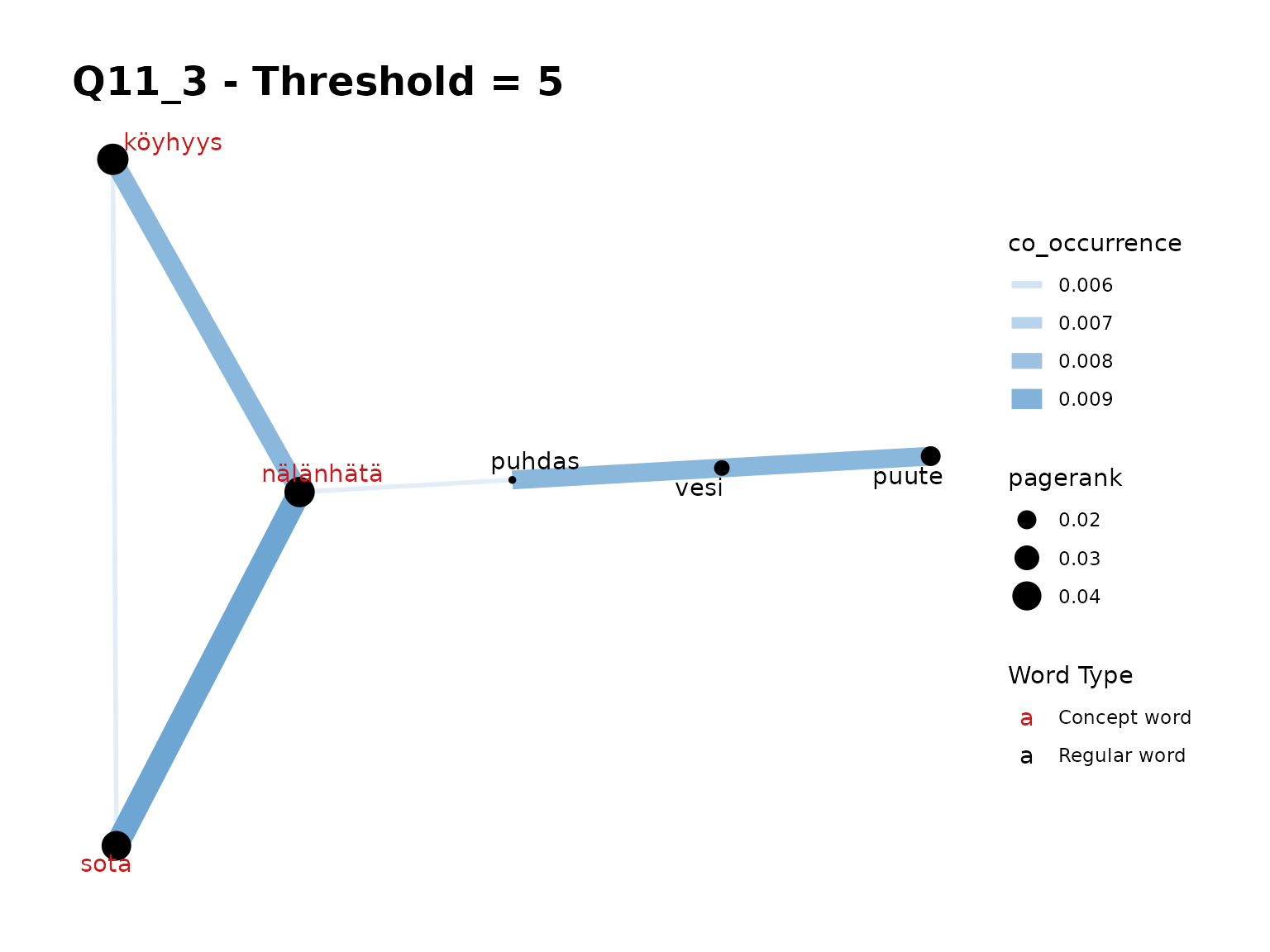
fst_concept_network(all_nltk,
  concepts = "köyhyys, nälänhätä, sota",
  threshold = 5,
  title = "Q11_3 - Threshold = 5",
  norm = "number_resp"
)

fst_concept_network(all_nltk,
  concepts = "köyhyys, nälänhätä, sota",
  threshold = 3,
  title = "Q11_3 - Threshold = 3",
  norm = "number_resp"
)

Remarks:

The ‘no threshold’ graph seems the most meaningful here.
We can see that our top three words, in red, are highly related to each other in use.
We can see the relationship between ‘vesi’ with ‘puute’ and ‘puhdas’ in this plot.

Now, let’s add more words in:

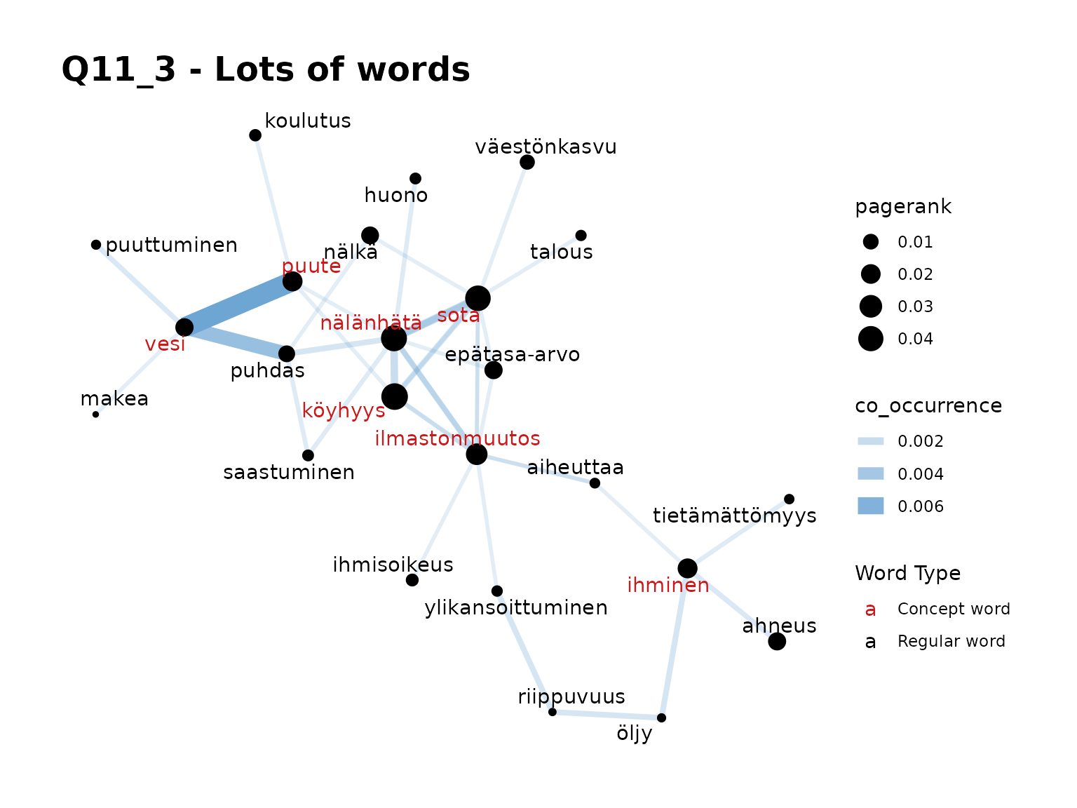
fst_concept_network(all_nltk,
  concepts = "köyhyys, nälänhätä, sota, ilmastonmuutos, puute, ihminen, vesi, epätasa-arvo",
  title = "Q11_3 - Lots of words",
  norm = "number_words"
)

fst_concept_network(all_nltk,
  concepts = "köyhyys, nälänhätä, sota, ilmastonmuutos, puute, ihminen, vesi, epätasa-arvo",
  title = "Q11_3 - Lots of words, threshold = 3", threshold = 5,
  norm = "number_resp"
)

Remarks:

The ‘no-threshold’ plot here is very busy. When we introduce a threshold, the plot splits in two which indicates that the two groups of words are only “connected” in a few responses.

Now, let’s see what do people who talk about water tend to also say in their responses:

fst_concept_network(all_nltk, concepts = "vesi", title = "Q11_3 - Vesi")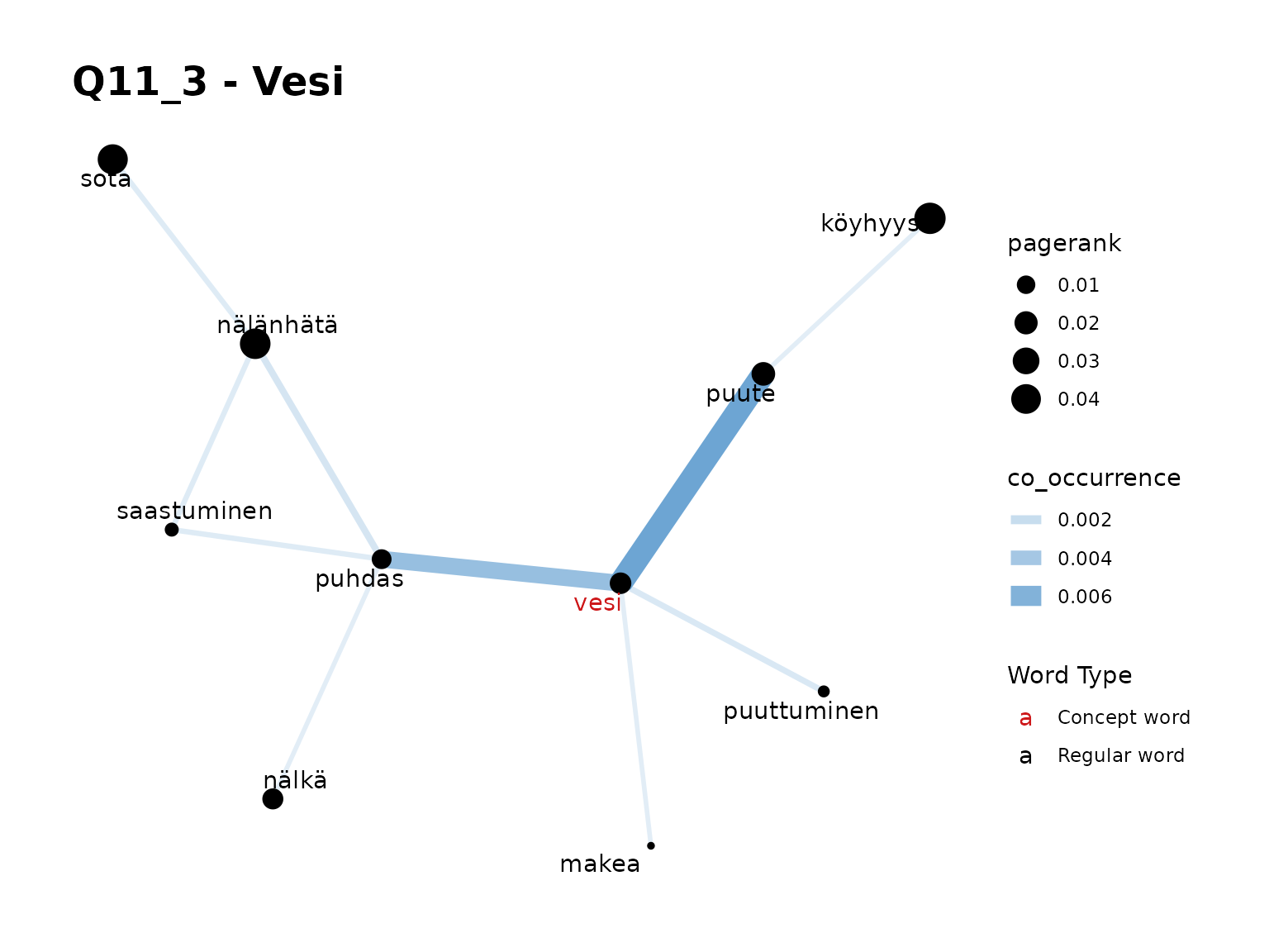

fst_concept_network(all_nltk, concepts = "puute, puhdas, vesi", title = "Q11_3 - ")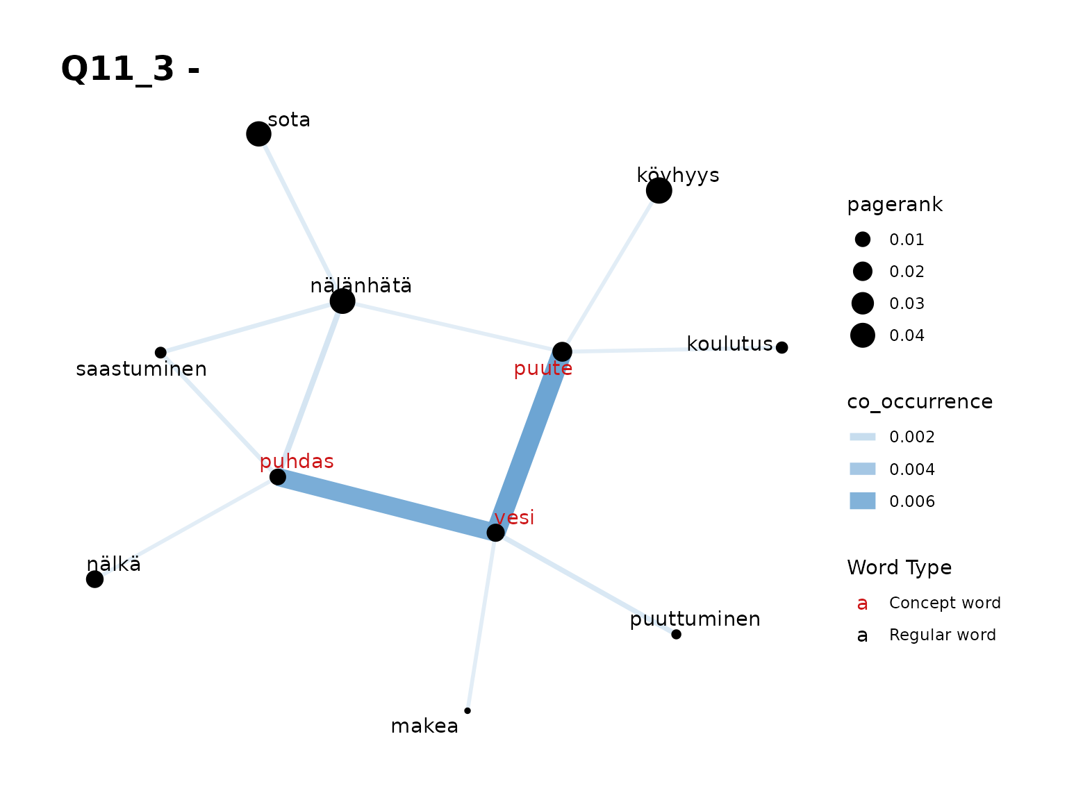

Remarks:

Again, we see the strong relationship with ‘puute’ and ‘puhdas’ with some other, less-frequent words too.

Comparison in responses split by gender

Now we’ve looked at responses as a whole, we consider whether gender impacts word choice. For further details on the comparison functions, please refer to “Tutorial5-Demonstration_of_comparison_functions”.

Summary Comparisons

We will start the comparison by looking at the summary functions:

knitr::kable(
  fst_summarise_compare(female_nltk, male_nltk, na_nltk, all_nltk, name1 = "F", name2 = "M", name3 = "NA", name4 = "All")
)

Description	Respondents	No Response	Proportion	Total Words	Unique Words	Unique Lemmas
F	673	13	0.98	2993	823	722
M	183	8	0.96	795	383	354
NA	89	4	0.96	404	225	208
All	945	25	0.97	4192	1132	994


knitr::kable(
  fst_pos_compare(female_nltk, male_nltk, na_nltk, all_nltk, name1 = "F", name2 = "M", name3 = "NA", name4 = "All")
)

UPOS	Part_of_Speech_Name	F Count	F Prop	M Count	M Prop	NA Count	NA Prop	All Count	All Prop
ADJ	adjective	276	0.092	69	0.087	44	0.109	389	0.093
ADP	adposition	19	0.006	3	0.004	2	0.005	24	0.006
ADV	adverb	44	0.015	11	0.014	9	0.022	64	0.015
NOUN	noun	2373	0.793	636	0.800	302	0.748	3311	0.790
NUM	numeral	1	0.000	1	0.001	3	0.007	5	0.001
PART	particle	18	0.006	8	0.010	3	0.007	29	0.007
PRON	pronoun	8	0.003	3	0.004	1	0.002	12	0.003
VERB	verb	195	0.065	45	0.057	38	0.094	278	0.066


knitr::kable(
  fst_length_compare(female_nltk, male_nltk, na_nltk, all_nltk, name1 = "F", name2 = "M", name3 = "NA", name4 = "All")
)

Description	Respondents	Mean	Minimum	Q1	Median	Q3	Maximum
F- Words	660	5.518182	1	4	5	6	28
F- Sentences	660	1.012121	1	1	1	1	3
M- Words	175	5.417143	2	4	5	6	32
M- Sentences	175	1.028571	1	1	1	1	3
NA- Words	85	5.694118	3	4	4	6	18
NA- Sentences	85	1.011765	1	1	1	1	2
All- Words	920	5.515217	1	4	5	6	32
All- Sentences	920	1.015217	1	1	1	1	3

Remarks:

Relatively consistent response rate, slightly higher (98%) response rate for females
Very consistent distribution across word type! - slightly less nouns (75%) in NA but this is a much smaller sample
Lengths of responses are similar across cohorts

Wordclouds

Now let’s consider the wordclouds. Let’s do comparison cloud and individual word clouds (we run a second comparison cloud without NA since this sample is so small)

fst_comparison_cloud(
  data1 = female_nltk, name1 = "Female",
  data2 = male_nltk, name2 = "Male",
  data3 = na_nltk, name3 = "NA",
  max = 50
)
#> Notes on use of fst_comparison_cloud: 
#>  If `max` is large, you may receive "warnings" indicating any words which are not plotted due to space constraints.
#> Note: 
#>  Consider whether your data is balanced between groups being compared and whether each group contains enough data for analysis. 
#>  The number of responses in each group (including 'NAs') are listed below: 
#>  Female=673, Male=183, NA=89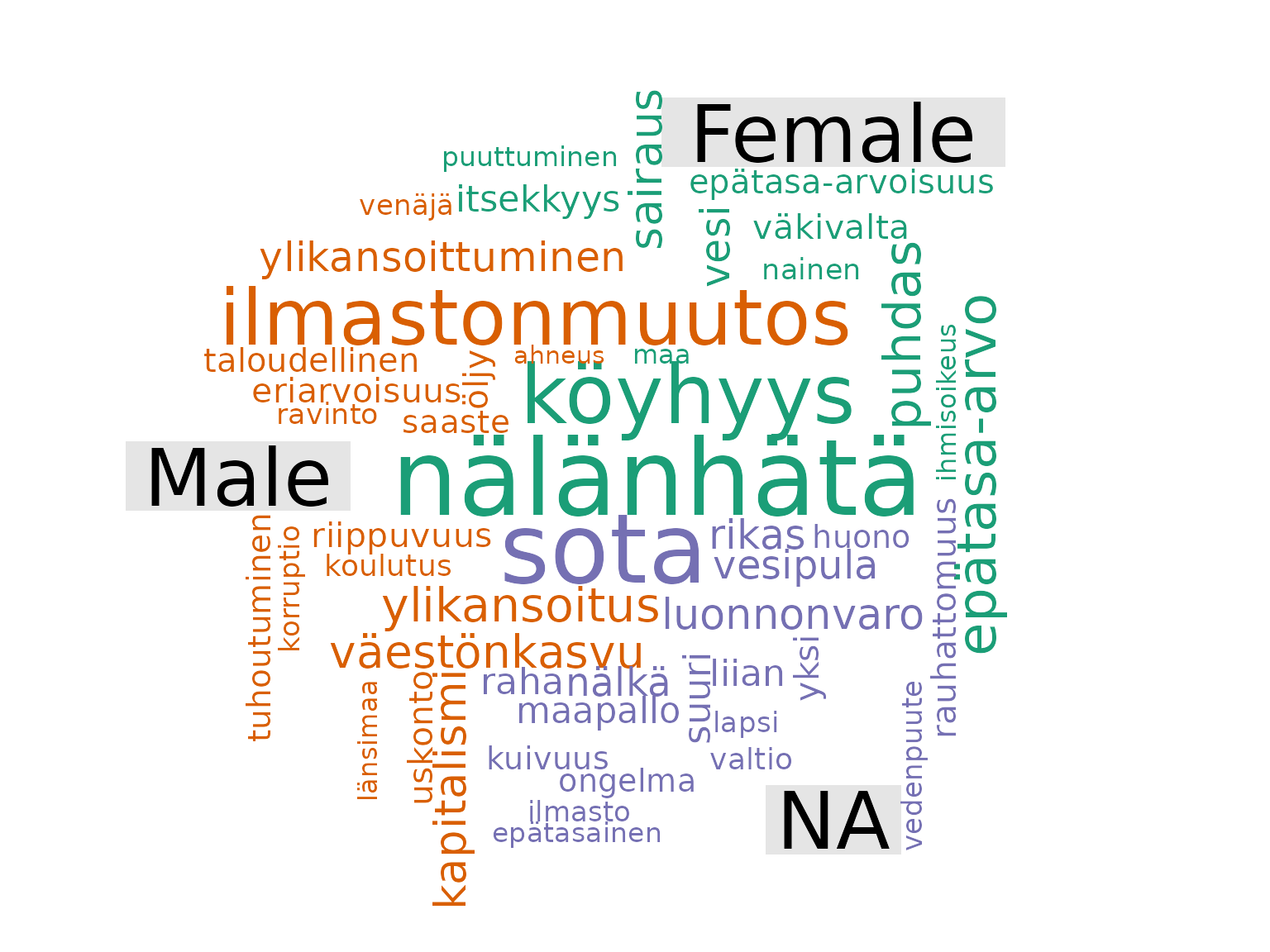


fst_comparison_cloud(
  data1 = female_nltk, name1 = "Female",
  data2 = male_nltk, name2 = "Male",
  max = 50
)
#> Notes on use of fst_comparison_cloud: 
#>  If `max` is large, you may receive "warnings" indicating any words which are not plotted due to space constraints.
#> Note: 
#>  Consider whether your data is balanced between groups being compared and whether each group contains enough data for analysis. 
#>  The number of responses in each group (including 'NAs') are listed below: 
#>  Female=673, Male=183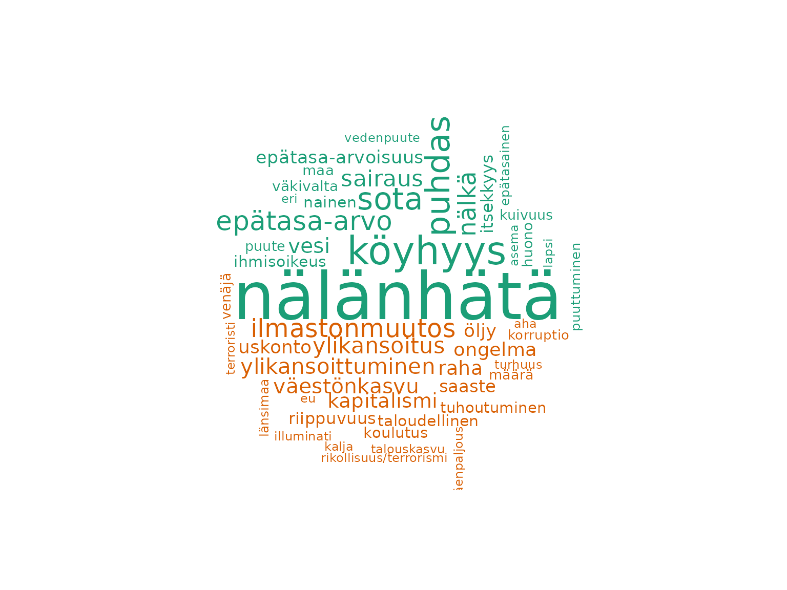


fst_wordcloud(female_nltk)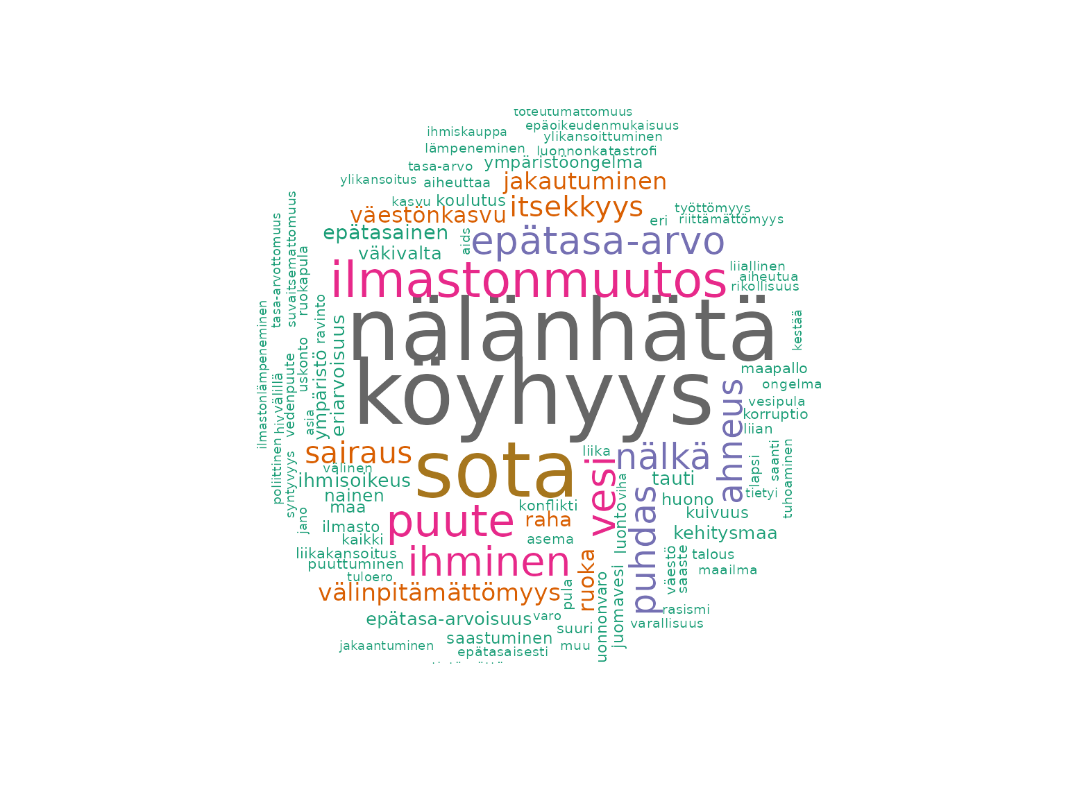

fst_wordcloud(male_nltk)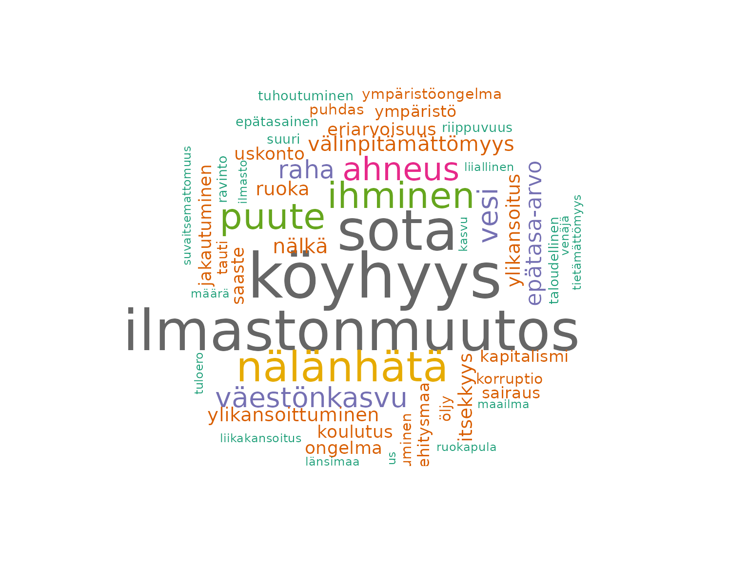

fst_wordcloud(na_nltk)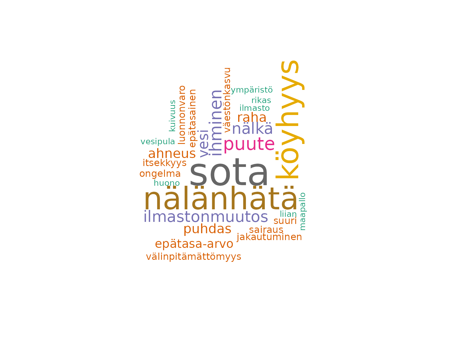

Based on comparison cloud, it looks like:

‘sota’ associated with those that didn’t provide a gender in their survey
‘epätasa-arvo’ ‘köyhyys’, and ’nälänhätä associated with females
‘ilmastonmuutos’ associated with males

When we look at individuals, we see:

‘ilmastonmuutos’ in top 3 for males - possibly # 2, nälänhätä less common for males
it’s evident we have less data for respondents who don’t list a gender. Their wordcloud is quite sparse!

N-grams and top words

Now we look at common words and n-grams. Here, we will exclude the responses with ‘NA’ for gender as we go on, as there are very few of these.

fst_freq_compare(
  data1 = female_nltk, name1 = "Female",
  data2 = male_nltk, name2 = "Male",
  data3 = na_nltk, name3 = "NA",
  number = 5,
  norm = "number_resp",
  pos_filter = NULL,
  unique_colour = "indianred",
  strict = TRUE
)
#> Note: 
#>  Consider whether your data is balanced between groups being compared and whether each group contains enough data for analysis. 
#>  The number of responses in each group (including 'NAs') are listed below: 
#>  Female=673, Male=183, NA=89
#> Note:
#>  Words with equal occurrence are presented in alphabetical order. 
#>  By default, words are presented in order to the `number` cutoff word. 
#>  This means that equally-occurring later-alphabetically words beyond the cutoff will not be displayed.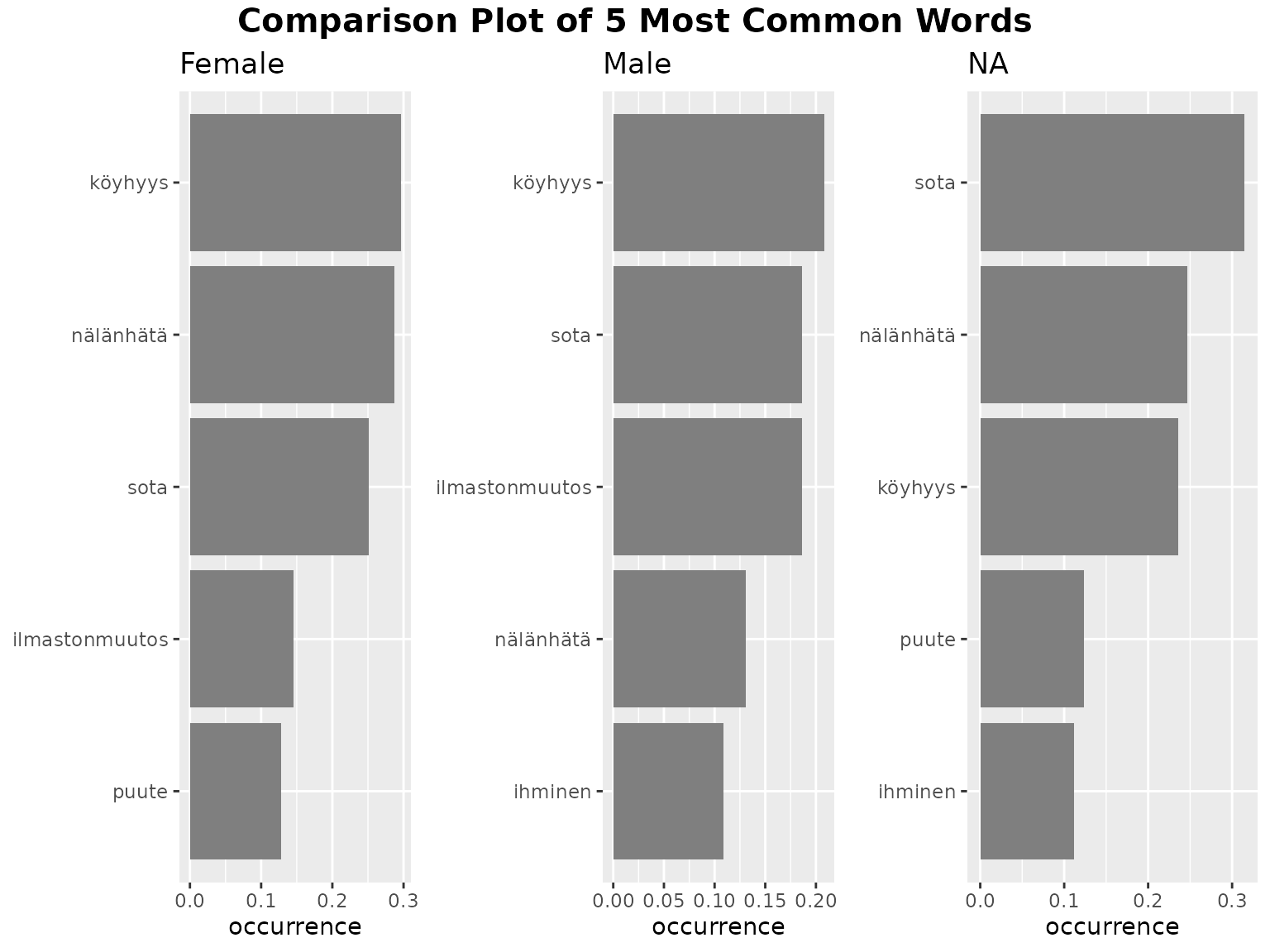


fst_freq_compare(
  data1 = female_nltk, name1 = "Female",
  data2 = male_nltk, name2 = "Male",
  number = 10,
  norm = "number_resp",
  pos_filter = NULL,
  unique_colour = "indianred",
  strict = TRUE
)
#> Note: 
#>  Consider whether your data is balanced between groups being compared and whether each group contains enough data for analysis. 
#>  The number of responses in each group (including 'NAs') are listed below: 
#>  Female=673, Male=183
#> 
#> 
#> Note:
#>  Words with equal occurrence are presented in alphabetical order. 
#>  By default, words are presented in order to the `number` cutoff word. 
#>  This means that equally-occurring later-alphabetically words beyond the cutoff will not be displayed.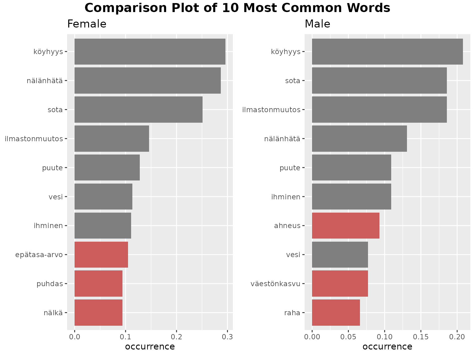



fst_ngrams_compare(
  data1 = female_nltk, name1 = "Female",
  data2 = male_nltk, name2 = "Male",
  number = 10,
  norm = "number_resp",
  ngrams = 2,
  pos_filter = NULL,
  unique_colour = "indianred",
  strict = TRUE
)
#> Note: 
#>  Consider whether your data is balanced between groups being compared and whether each group contains enough data for analysis. 
#>  The number of responses in each group (including 'NAs') are listed below: 
#>  Female=673, Male=183
#> Note:
#>  N-grams with equal occurrence are presented in alphabetical order. 
#>  By default, n-grams are presented in order to the `number` cutoff n-gram 
#>  This means that equally-occurring later-alphabetically n-grams beyond the cutoff n-gram will not be displayed.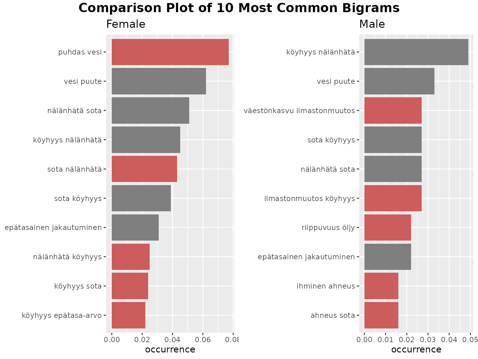

Remarks:

Here we see that male and female respondents have the same top 4 words, but that ‘nälänhätä’ is more frequent for females than males, and ‘ilmastonmuutos’ conversely. This may prompt further research into whether male survey participants show more concern about climate change than females in the remainder of the survey.

Also, we note that the most frequent words by female respondents occur in nearly 30% of responses whereas for the males it’s just over 20%. Perhaps there is less consistency in what males are mentioning?

For the bigrams, we can identify that

both genders frequently list lack of water but it is mostly females who mention clean water.

Concept Network of top 4 words

Now, we’ll look at the Concept Network for the 4 top words in female and male responses. These words are ‘sota’, ‘köyhyys’, nälänhätä’, and ‘ilmastonmuutos’.

fst_concept_network_compare(
  data1 = female_nltk, name1 = "Female",
  data2 = male_nltk, name2 = "Male",
  concepts = "köyhyys, nälänhätä, sota, ilmastonmuutos", threshold = 1
)
#> Note: 
#>  Consider whether your data is balanced between groups being compared and whether each group contains enough data for analysis. 
#>  The number of responses in each group (including 'NAs') are listed below: 
#>  Female=673, Male=183

Remarks:

Interestingly, our Concept Network plots of these top 4 words show that there is a much larger variety of terms used by female respondents who mention these 4 common responses.

Only part of this is explained by the fact that we have nearly 4 times as many responses from female participants since each of these plots have their vertex weights determined from only their cohort’s responses. Therefore, there may be other subgroups within the male respondents who discuss independent themes to these.

Conclusion

This tutorial demonstrates the use of finnsurveytext to look at a single question and then consider whether gender impacts response. Gender is just one of many ways you could split the data and is used as an example in this context. It is likely an analyst would also want to split the data in other ways such as age, education level, etc.

Following the use of finnsurveytext, we have a number of hypotheses, such as “Male survey respondents are more concerned about climate change than females”, which could inform further analysis of the survey as a whole.

Citation

Finnish Children and Youth Foundation: Young People’s Views on Development Cooperation 2012 [dataset]. Version 2.0 (2019-01-22). Finnish Social Science Data Archive [distributor]. http://urn.fi/urn:nbn:fi:fsd:T-FSD2821

Tutorial6-Example_of_analysis_of_an_open-ended_survey_question

Introduction

Installation of package.

The Question

Overview of Functions

The Data

Development Cooperation Data Split by Gender

Analysis

Translations

Top N-Grams

A Concept Network

Comparison in responses split by gender

Summary Comparisons

Wordclouds

N-grams and top words

Concept Network of top 4 words

Conclusion

Citation