Tutorial5-Demonstration_of_comparison_functions

Introduction

When analysing responses to open-ended questions, you may want to look into whether different groups of survey participants have, in general, responded differently to the prompt. finnsurveytext contains a number of comparison functions which are intended to be used to compare responses between groups. These comparison functions covered are defined in r/04_comparison_functions.R and r/05_comparison_concept_network.R.

One way to split the data is using a different question within the survey such as a categorical question (eg. gender, location, or level of education) or an ordinal variable (such as age or income bracket). In this tutorial, we will look at comparing responses to a question based on gender. Before using the comparison functions, we run the preparation functions which are in r/01_prepare_conll-u.R (and which are covered in detail in ‘Tutorial1-Prepare CoNLL-U’) for each group separately.

The comparison functions are:

1. fst_summarise_compare()
2. fst_pos_compare()
3. fst_length_compare()
4. fst_comparisoncloud()
5. fst_get_unique_ngrams()
6. fst_join_unique()
7. fst_ngrams_compare_plot()
8. fst_ngrams_compare_plot2()
9. fst_plot_multiple()
10. fst_freq_compare()
11. fst_ngrams_compare()
12. fst_cn_get_unique()
13. fst_cn_compare_plot()
14. fst_concept_network_compare()

We will look at the following question:

• q11_2] Jatka lausetta: Kehitysyhteistyö on toimintaa, jossa… (Avokysymys)
  • (In English) q11_2] Continue the sentence: Development cooperation is an activity in which… (Open question)

Installation of package.

Once the package is installed, you can load the finnsurveytext package as below: (Other required packages such as dplyr and stringr will also be installed if they are not currently installed in your environment.)

library(finnsurveytext)

The Data

There are four sets of data files available within the package which are used in this tutorial

Development Cooperation Data Split by Gender

• data/dev_data.rda - All responses to the survey
• data/dev_data_m.rda - Responses to the survey by participants who have listed their gender as male
• data/dev_data_f.rda - Responses to the survey by participants who have listed their gender as female
• data/dev_data_na.rda - Responses to the survey by participants who have not responded to the gender question

We can prepare the data into CoNLL-U format using functions from 01_prepare_conllu-u.R as follows: (We are preparing versions with and without stopwords removed because we have some functions which are more informative with or without the stopwords included.)

all <- fst_prepare_conllu(
  data = dev_data,
  field = "q11_2",
  stopword_list = "none"
)

all_nltk <- fst_prepare_conllu(
  data = dev_data,
  field = "q11_2",
  stopword_list = "nltk"
)

female <- fst_prepare_conllu(
  data = dev_data_f,
  field = "q11_2",
  stopword_list = "none"
)

female_nltk <- fst_prepare_conllu(
  data = dev_data_f,
  field = "q11_2",
  stopword_list = "nltk"
)

male <- fst_prepare_conllu(
  data = dev_data_m,
  field = "q11_2",
  stopword_list = "none"
)

male_nltk <- fst_prepare_conllu(
  data = dev_data_m,
  field = "q11_2",
  stopword_list = "nltk"
)

na <- fst_prepare_conllu(
  data = dev_data_na,
  field = "q11_2",
  stopword_list = "none"
)

na_nltk <- fst_prepare_conllu(
  data = dev_data_na,
  field = "q11_2",
  stopword_list = "nltk"
)

The data is formatted like this:

knitr::kable(head(male_nltk))

doc_id	paragraph_id	sentence_id	sentence	token_id	token	lemma	upos	xpos	feats	head_token_id	dep_rel	deps	misc
doc1	1	1	parannetaan kehitysmaiden oloja.	1	parannetaan	paranneta	VERB	V,Pass,Ind,Pres	Mood=Ind|Tense=Pres|VerbForm=Fin|Voice=Pass	0	root	NA	NA
doc1	1	1	parannetaan kehitysmaiden oloja.	2	kehitysmaiden	kehitysmaa	NOUN	N,Pl,Gen	Case=Gen|Number=Plur	3	nmod	NA	NA
doc1	1	1	parannetaan kehitysmaiden oloja.	3	oloja	olo	NOUN	N,Pl,Par	Case=Par|Number=Plur	1	obj	NA	SpaceAfter=No
doc2	1	1	NA	1	na	na	NOUN	N,Sg,Par	Case=Par|Number=Sing	0	root	NA	SpacesAfter=
doc3	1	1	autetaan parantamaan kehitysmaiden oloja	1	autetaan	auttaa	VERB	V,Pass,Ind,Pres	Mood=Ind|Tense=Pres|VerbForm=Fin|Voice=Pass	0	root	NA	NA
doc3	1	1	autetaan parantamaan kehitysmaiden oloja	2	parantamaan	parantaa	VERB	V,Act,InfMa,Ill	Case=Ill|InfForm=3|VerbForm=Inf|Voice=Act	1	xcomp	NA	NA

Now that our data is ready, we can look at our data and compare the results.

Comparison of responses based on gender

All of our comparison functions can compare between two and four sets of data. The following common arguments appear in multiple functions and are defined the same way in each:

• data1, data2, data3 and data4 are the processed data in ConLL-U format (such as the output of fst_prepare_connlu) for the groups for comparison. Since you can compare between 2 and 4 groups, data3 and data4 are both optional.
• name1, name2, name3 and name4 are optional descriptive names for the different groups. They will default to "Group 1", "Group 2", "Group 3", and "Group 4".

First, we will look at some summary functions to compare the responses overall. (We are using the versions which include the stopwords here.) The functions are:

1. fst_summarise_compare()
2. fst_pos_summary()
3. fst_length_compare()

Make Comparison Summary

We can run this function to create a summary table for our data: (we use knitr::kable function below to display results in a “prettier” table)

knitr::kable(
  fst_summarise_compare(
    data1 = all, name1 = "All",
    data2 = female, name2 = "Female",
    data3 = male, name3 = "Male",
    data4 = na, name4 = "Unspecified"
  )
)

Description	Respondents	No Response	Proportion	Total Words	Unique Words	Unique Lemmas
All	945	34	0.97	5495	1357	932
Female	673	18	0.97	4102	1062	738
Male	183	8	0.96	965	440	339
Unspecified	89	8	0.92	428	214	178

To run fst_summarise_compare(), we provide the following arguments to the function:

• data1, data2, data3 and data4 (as defined above, data3 and data4 are optional)
• name1, name2, name3 and name4 (optional, as defined above)

Remarks:

We can already see that our data is quite unbalanced. There are a lot more female respondents than male or unspecified. The response (to this question) rate is high (97%) but slightly lower for the unspecified respondents. Unsurprisingly, since there are more female responses, the female responses to this question contain a larger variety of words.

POS and Length Comparisons

Next, we will look at part-of-speech tags and lengths of responses.

knitr::kable(
  fst_pos_compare(
    data1 = all, name1 = "All",
    data2 = female, name2 = "Female",
    data3 = male, name3 = "Male",
    data4 = na, name4 = "Unspecified"
  )
)

UPOS	Part_of_Speech_Name	All Count	All Prop	Female Count	Female Prop	Male Count	Male Prop	Unspecified Count	Unspecified Prop
ADJ	adjective	353	0.064	275	0.067	59	0.061	19	0.044
ADP	adposition	72	0.013	52	0.013	17	0.018	3	0.007
ADV	adverb	187	0.034	141	0.034	33	0.034	13	0.030
AUX	auxiliary	65	0.012	42	0.010	20	0.021	3	0.007
CCONJ	coordinating conjunction	237	0.043	179	0.044	38	0.039	20	0.047
DET	determiner	116	0.021	88	0.021	23	0.024	5	0.012
NOUN	noun	1976	0.360	1449	0.353	356	0.369	171	0.400
PART	particle	64	0.012	51	0.012	6	0.006	7	0.016
PRON	pronoun	114	0.021	78	0.019	24	0.025	12	0.028
PUNCT	punctuation	591	0.108	450	0.110	102	0.106	39	0.091
SCONJ	subordinating conjunction	20	0.004	16	0.004	3	0.003	1	0.002
VERB	verb	1683	0.306	1268	0.309	281	0.291	134	0.313

knitr::kable(
  fst_length_compare(
    data1 = all, name1 = "All",
    data2 = female, name2 = "Female",
    data3 = male, name3 = "Male",
    data4 = na, name4 = "Unspecified",
    incl_sentences = TRUE
  )
)

Description	Respondents	Mean	Minimum	Q1	Median	Q3	Maximum
All- Words	911	5.374314	0	3	4	7	30
All- Sentences	911	1.018661	1	1	1	1	3
Female- Words	655	5.578626	0	3	4	7	30
Female- Sentences	655	1.021374	1	1	1	1	3
Male- Words	175	4.914286	0	3	4	6	21
Male- Sentences	175	1.011429	1	1	1	1	2
Unspecified- Words	81	4.716049	1	3	4	6	13
Unspecified- Sentences	81	1.012346	1	1	1	1	2

Both these functions have the same arguments, as defined above:

• data1, data2, data3 and data4 (data3 and data4 are optional)
• name1, name2, name3 and name4

Additionally, fst_length_compare() has:

• incl_sentences an optional boolean of whether to include sentence data in table, default is TRUE. If incl_sentences = TRUE, the table will also provide length information for the number of sentences within responses. If incl_sentences = FALSE, the table will show only show results for the number of words in responses.

Remarks:

In terms of POS tags, the scale differences are likely mostly due to the differences in the number of respondents between genders. We can also see that female responses are generally slightly longer (average of 6 words to 5 words) but that most respondents (across the genders) wrote only a single sentence.

Comparison Cloud

Now that we’ve looked at the overview comparisons, we will create a comparison cloud between the responses, using the versions with stopwords removed so that only more meaningful words remain.

A comparison cloud compares the relative frequency with which a term is used in two or more documents. This cloud shows words that occur more regularly in responses from a specific type of respondent. For more information about comparison clouds, you can read this documentation.

We create our comparison cloud as follows:

fst_comparison_cloud(
  data1 = female, name1 = "Female",
  data2 = male, name2 = "Male",
  data3 = na, name3 = "Unspecified",
  pos_filter = NULL,
  max = 50
)
#> Notes on use of fst_comparison_cloud: 
#>  If `max` is large, you may receive "warnings" indicating any words which are not plotted due to space constraints.
#> Note: 
#>  Consider whether your data is balanced between groups being compared and whether each group contains enough data for analysis. 
#>  The number of responses in each group (including 'NAs') are listed below: 
#>  Female=673, Male=183, Unspecified=89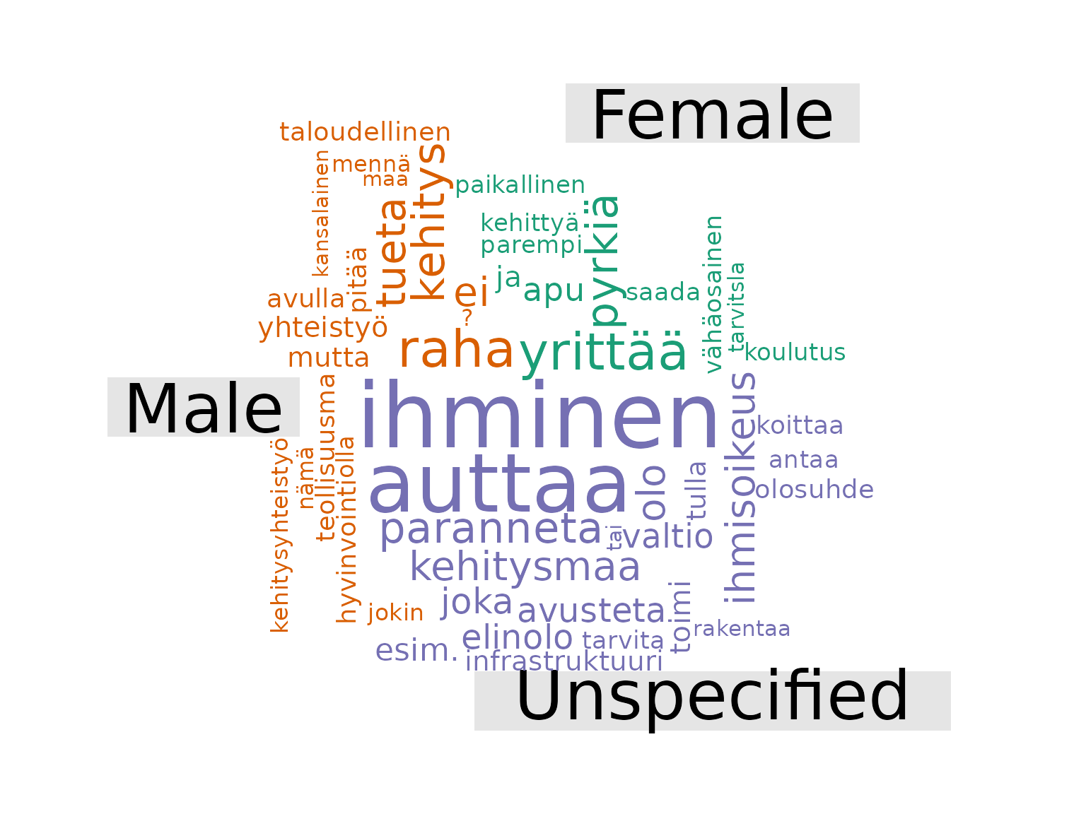

To run fst_comparison_cloud(), we provide the following arguments to the function:

• data1, data2, data3 and data4 (as defined above, data3 and data4 are optional)
• name1, name2, name3 and name4 (optional, as defined above)
• pos_filter is an optional list of POS tags for inclusion in the wordcloud. The defaul is NULL.
• max is the maximum number of words to display, the default is 100.

Remarks:

Our data is quite unbalanced (there are a lot more female respondents and fewer ‘NA’ so this may skew responses) but it seems that a higher proportion of these ‘NA’ respondents use ‘ihminen’ and ‘auttaa’ in their responses. Similarly, ‘raha’ and ‘yrittää’ are associated with males and females respectively.

Common Words and N-grams

Now, we will look at common words occurring in the responses.

First, we will consider all the responses for this question. We are not filtering the data based on POS tag, and will leave the default of strict = TRUE which will cut-off the list at 10 words (see the warning note about this). We also use the default for the norm which means we are standardising between groups by dividing count of a word by the total number of words in the responses.

For definition of fst_get_top_words() and fst_get_top_ngrams() functions, see “Tutorial2-Data_Exploration”.

all_top10 <- fst_get_top_words(all_nltk,
  number = 10,
  norm = "number_words",
  pos_filter = NULL,
  strict = FALSE
)
#> Note:
#>  Words with equal occurrence are presented in alphabetical order. 
#>  With `strict` = FALSE, words occurring equally often as the `number` cutoff word will be displayed.
all_top10bigrams <- fst_get_top_ngrams(all_nltk,
  number = 10,
  ngrams = 2,
  norm = "number_words",
  pos_filter = NULL,
  strict = TRUE
)
#> Note:
#>  N-grams with equal occurrence are presented in alphabetical order. 
#>  By default, n-grams are presented in order to the `number` cutoff n-gram. 
#>  This means that equally-occurring later-alphabetically n-grams beyond the cutoff n-gram will not be displayed.

knitr::kable(all_top10)

words	occurrence
kehitysmaa	0.106
auttaa	0.105
pyrkiä	0.046
maa	0.035
ihminen	0.032
parantaa	0.030
yrittää	0.021
olo	0.017
tueta	0.013
kehittää	0.012

knitr::kable(all_top10bigrams)

words	occurrence
auttaa kehitysmaa	0.044
pyrkiä auttaa	0.013
pyrkiä parantaa	0.012
kehitysmaa auttaa	0.011
parantaa kehitysmaa	0.010
kehitysmaa ihminen	0.009
kehitysmaa olo	0.008
yrittää auttaa	0.008
kehitysmaa pyrkiä	0.007
maa auttaa	0.006

Now we will look at top words by gender:

female_top10 <- fst_get_top_words(female_nltk,
  number = 10,
  norm = "number_words",
  pos_filter = NULL,
  strict = TRUE
)
#> Note:
#>  Words with equal occurrence are presented in alphabetical order. 
#>  By default, words are presented in order to the `number` cutoff word. 
#>  This means that equally-occurring later-alphabetically words beyond the cutoff word will not be displayed.
knitr::kable(female_top10)

words	occurrence
auttaa	0.111
kehitysmaa	0.106
pyrkiä	0.048
ihminen	0.034
maa	0.033
parantaa	0.030
yrittää	0.024
olo	0.017
apu	0.013
kehittää	0.012

male_top10 <- fst_get_top_words(male_nltk,
  number = 10,
  norm = "number_words",
  pos_filter = NULL,
  strict = TRUE
)
#> Note:
#>  Words with equal occurrence are presented in alphabetical order. 
#>  By default, words are presented in order to the `number` cutoff word. 
#>  This means that equally-occurring later-alphabetically words beyond the cutoff word will not be displayed.
knitr::kable(male_top10)

words	occurrence
kehitysmaa	0.104
auttaa	0.073
pyrkiä	0.042
maa	0.039
parantaa	0.027
tueta	0.021
raha	0.018
ihminen	0.017
kehitys	0.014
yhteistyö	0.014

na_top10 <- fst_get_top_words(na_nltk,
  number = 10,
  norm = "number_words",
  pos_filter = NULL,
  strict = TRUE
)
#> Note:
#>  Words with equal occurrence are presented in alphabetical order. 
#>  By default, words are presented in order to the `number` cutoff word. 
#>  This means that equally-occurring later-alphabetically words beyond the cutoff word will not be displayed.
knitr::kable(na_top10)

words	occurrence
auttaa	0.111
kehitysmaa	0.111
ihminen	0.048
maa	0.037
pyrkiä	0.034
parantaa	0.028
olo	0.023
paranneta	0.014
antaa	0.011
elinolo	0.011

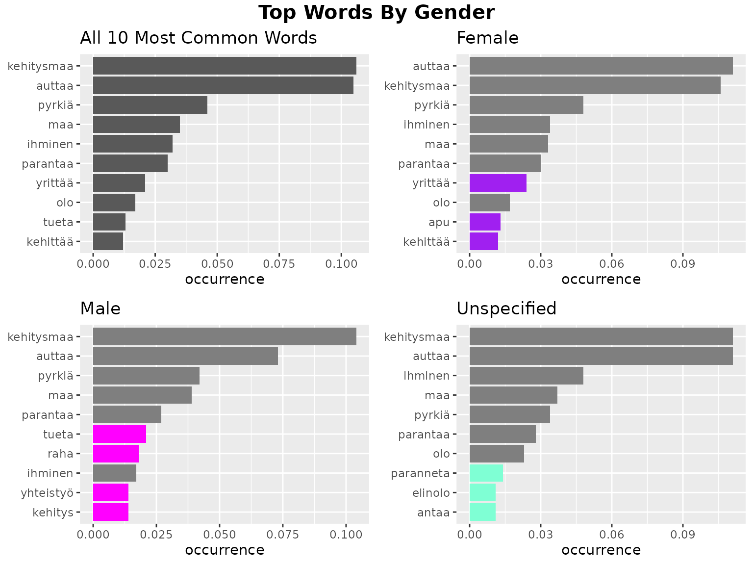
Remarks:

As you can see, the top words are very similar across all respondent types.

Comparison N-Gram Plots

This is further shown in the comparison plots. There are two functions which create the plots in one function simply. These are fst_freq_compare() and fst_ngrams_compare().

(Note that words that are unique to a gender are highlighted in red. This is only comparing the top 10 words, so be aware this word likely still appears in the other genders, just less frequently!)

fst_freq_compare(
  data1 = female_nltk, name1 = "Female",
  data2 = male_nltk, name2 = "Male",
  data3 = na_nltk, name3 = "Unspecified",
  number = 10,
  norm = "number_words",
  pos_filter = NULL,
  unique_colour = "indianred",
  strict = TRUE
)
#> Note: 
#>  Consider whether your data is balanced between groups being compared and whether each group contains enough data for analysis. 
#>  The number of responses in each group (including 'NAs') are listed below: 
#>  Female=672, Male=180, Unspecified=89
#> Note:
#>  Words with equal occurrence are presented in alphabetical order. 
#>  By default, words are presented in order to the `number` cutoff word. 
#>  This means that equally-occurring later-alphabetically words beyond the cutoff will not be displayed.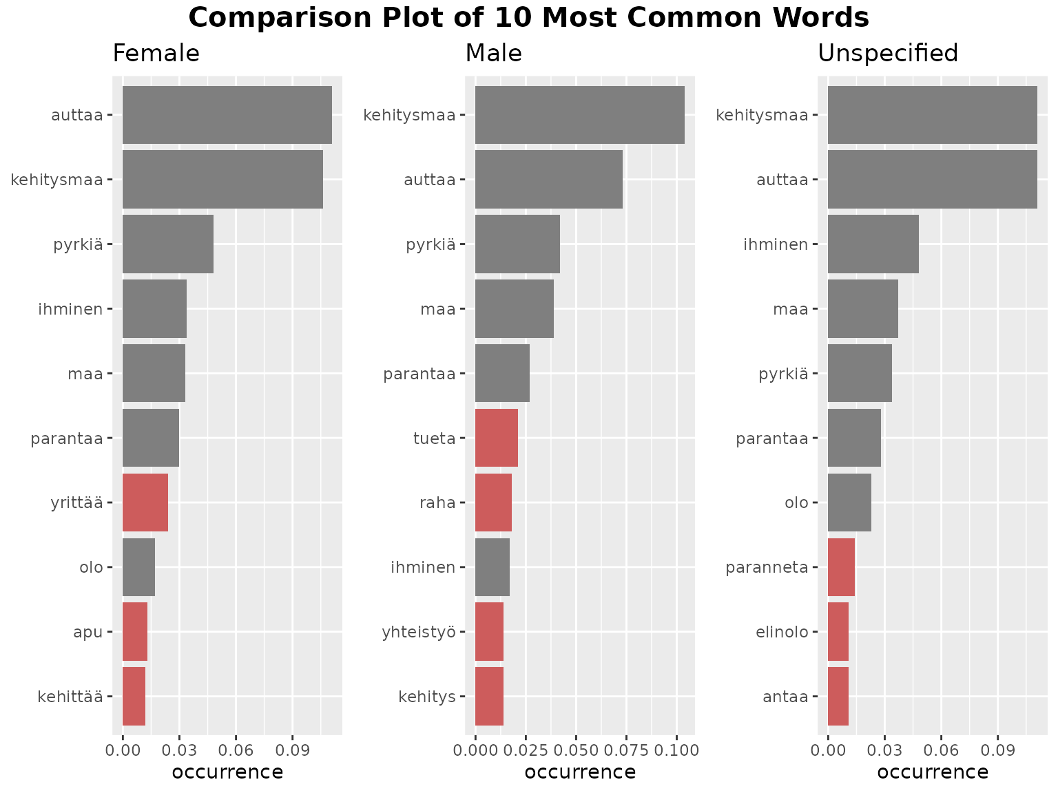

The function fst_freq_compare() has the following arguments:

• data1, data2, data3 and data4 (as defined above, data3 and data4 are optional)
• name1, name2, name3 and name4 (optional, as defined above)
• number is the number of top words to return, default is 10.
• norm is the method for normalising the data. Valid settings are 'number_words' (the number of words in the responses, default), 'number_resp' (the number of responses), or NULL (raw count returned).
• pos_filter is an optional list of which POS tags to include such as 'c("NOUN", "VERB", "ADJ", "ADV")'. The default is NULL, in which case all words in the data are considered.
• unique_colour is the colour that unique words will be displayed, the default is indianred.
• strict is a boolean that determines how the function will deal with ‘ties’. If strict = TRUE, the table will cut-off at the exact number(words are presented in alphabetical order so later-alphabetically, equally occurring words to the word at number will not be shown.) If strict = FALSE, the table will show any words that occur equally frequently as the number cutoff word.

fst_ngrams_compare(
  data1 = female_nltk, name1 = "Female",
  data2 = male_nltk, name2 = "Male",
  data3 = na_nltk, name3 = "Unspecified",
  number = 10,
  ngrams = 2,
  norm = "number_words",
  pos_filter = NULL,
  unique_colour = "indianred",
  strict = TRUE
)
#> Note: 
#>  Consider whether your data is balanced between groups being compared and whether each group contains enough data for analysis. 
#>  The number of responses in each group (including 'NAs') are listed below: 
#>  Female=672, Male=180, Unspecified=89
#> Note:
#>  N-grams with equal occurrence are presented in alphabetical order. 
#>  By default, n-grams are presented in order to the `number` cutoff n-gram 
#>  This means that equally-occurring later-alphabetically n-grams beyond the cutoff n-gram will not be displayed.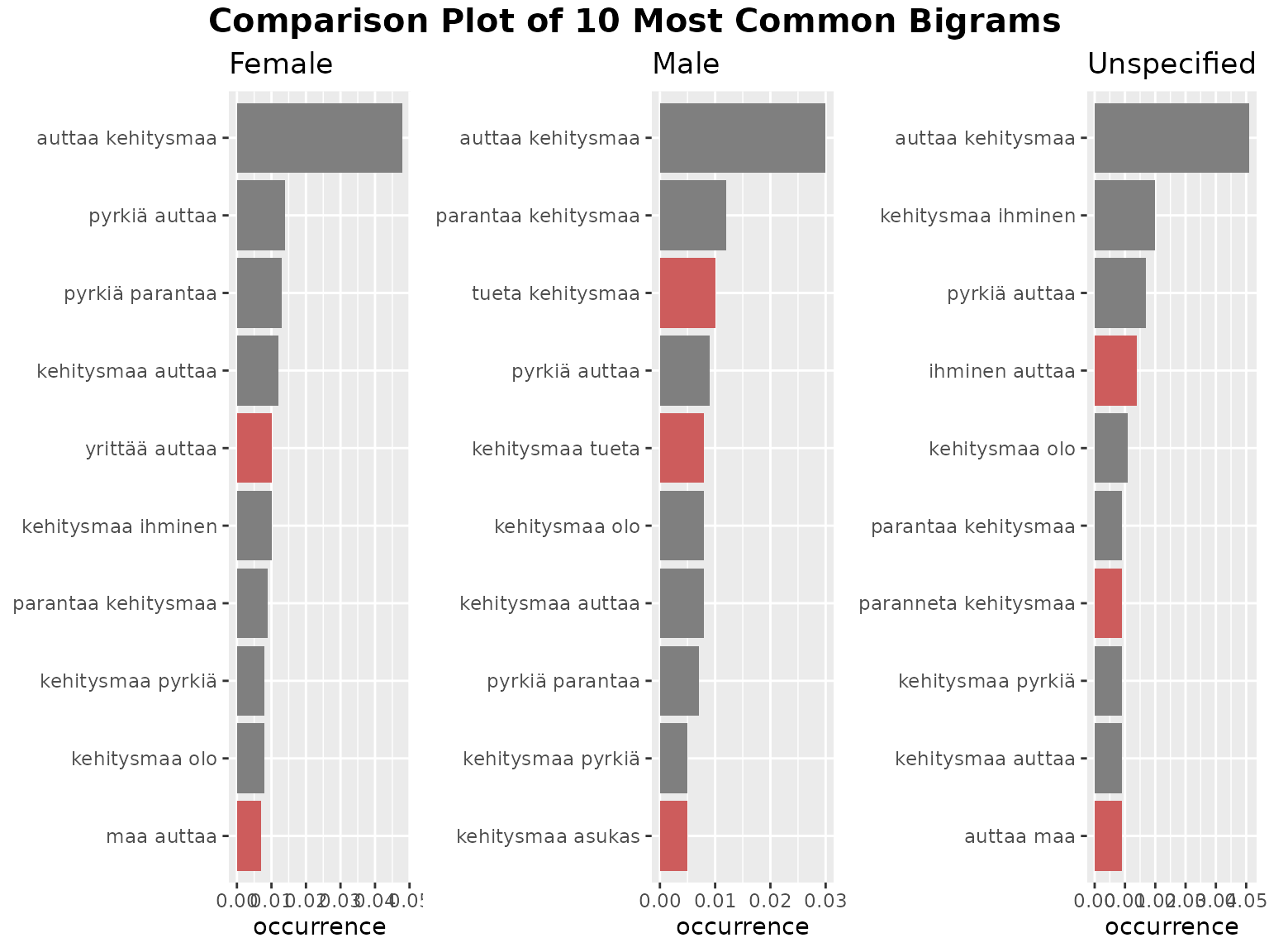

The function fst_ngrams_compare() has the following arguments:

• data1, data2, data3 and data4 (as defined above, data3 and data4 are optional)
• name1, name2, name3 and name4 (optional, as defined above)
• number is the number of top words to return, default is 10.
• ngrams is the type of n-grams. The default is “1” (so top words). Set ngrams = 2 to get bigrams and n = 3 to get trigrams etc.
• norm is the method for normalising the data. Valid settings are 'number_words' (the number of words in the responses, default), 'number_resp' (the number of responses), or NULL (raw count returned).
• pos_filter is an optional list of which POS tags to include such as 'c("NOUN", "VERB", "ADJ", "ADV")'. The default is NULL, in which case all words in the data are considered.
• unique_colour is the colour that unique words will be displayed, the default is indianred.
• strict is a boolean that determines how the function will deal with ‘ties’. If strict = TRUE, the table will cut-off at the exact number(words are presented in alphabetical order so later-alphabetically, equally occurring words to the word at number will not be shown.) If strict = FALSE, the table will show any words that occur equally frequently as the number cutoff word.

Now, we might want to compare this to the overall results. Since, fst_freq_compare() looks for unique words among all the sets provided, and we only want to look for unique words within the gender-specific sets, we need to run this activity through the component functions. These are fst_get_unique_ngrams(), fst_join_unique(), fst_ngrams_compare_plot() and fst_plot_multiple(). (Just for fun, let’s also changed the colour of the unique words.)

unique <- fst_get_unique_ngrams(female_top10, male_top10, na_top10)

female_top10u <- fst_join_unique(female_top10, unique)
male_top10u <- fst_join_unique(male_top10, unique)
na_top10u <- fst_join_unique(na_top10, unique)

plot_all <- fst_freq_plot(all_top10, number = 10, name = "All")
plot_f <- fst_ngrams_compare_plot(female_top10u,
  ngrams = 1,
  number = 10,
  override_title = "Female",
  unique_colour = "purple"
)
plot_m <- fst_ngrams_compare_plot(male_top10u,
  ngrams = 1,
  number = 10,
  override_title = "Male",
  unique_colour = "magenta"
)
plot_na <- fst_ngrams_compare_plot(na_top10u,
  ngrams = 1,
  number = 10,
  override_title = "Unspecified",
  unique_colour = "aquamarine"
)

fst_plot_multiple(plot_all,
  plot_f,
  plot_m,
  plot_na,
  main_title = "Top Words By Gender"
)

The arguments of these functions are:

• fst_get_unique_ngrams():
  • table1, table2, … - A list of names of tables which are the output of fst_get_top_words() or fst_get_top_ngrams()
• fst_join_unique():
  • table is a table that is the output of fst_get_top_words() or fst_get_top_ngrams()
  • unique is the output of fst_get_unique_ngrams()
• fst_ngrams_compare_plot():
  • table is the table of words/n-grams, output of fst_join_unique()
  • number is the number of n-grams, default is 10.
  • ngrams is the type of n-grams, default is 1.
  • unique_colouris the colour to display unique words, default is "indianred".
  • name is an optional “name” for the plot, default is NULL
• fst_plot_multiple():
  • plot1, plot2, plot3 and plot4 are the plots. Since you can compare between 2 and 4 plots, plot3 and plot4 are both optional.

Comparison Concept Network

Since the top 3 words are ‘kehitysmaa’, ‘auttaa’, and ‘pyrkiä’, we will create Concept Networks based on these terms.

We run the comparison Concept Network as below. Again, we’re keeping the default norm.

fst_concept_network_compare(
  data1 = female_nltk, name1 = "Female",
  data2 = male_nltk, name2 = "Male",
  data3 = na_nltk, name3 = "Unspecified",
  concepts = "kehitysmaa, auttaa, pyrkiä"
)
#> Note: 
#>  Consider whether your data is balanced between groups being compared and whether each group contains enough data for analysis. 
#>  The number of responses in each group (including 'NAs') are listed below: 
#>  Female=672, Male=180, Unspecified=89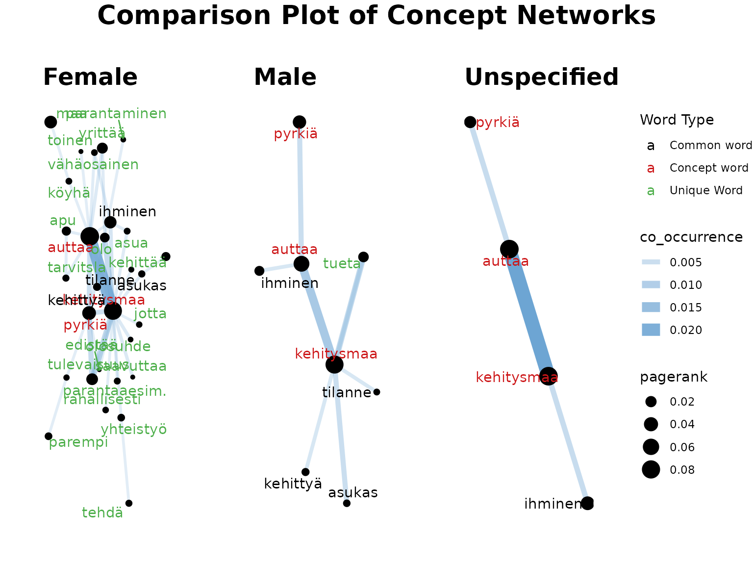

The arguments are:

• data1, data2, data3 and data4 (as defined above, data3 and data4 are optional)
• name1, name2, name3 and name4 (optional, as defined above)
• pos_filter is a list of UPOS tags for inclusion, default is NULL.
• concepts is a string of concept terms to search for, separated by commas.
• norm is the method for normalising the data. Valid settings are 'number_words' (the number of words in the responses, default), 'number_resp' (the number of responses), or NULL (raw count returned). Normalisation occurs after the threshold (if it exists) is applied.
• threshold is the minimum number of occurrences threshold for ‘edge’ between a concept term and other word, default is NULL.

Remarks:

As you can see, this can result in a plot that is too busy (especially in the markdown format where we’ve limited the size of the plots).

Let’s try again with just male and female data.

fst_concept_network_compare(
  data1 = female_nltk, name1 = "Female",
  data2 = male_nltk, name2 = "Male",
  concepts = "kehitysmaa, auttaa, pyrkiä"
)
#> Note: 
#>  Consider whether your data is balanced between groups being compared and whether each group contains enough data for analysis. 
#>  The number of responses in each group (including 'NAs') are listed below: 
#>  Female=672, Male=180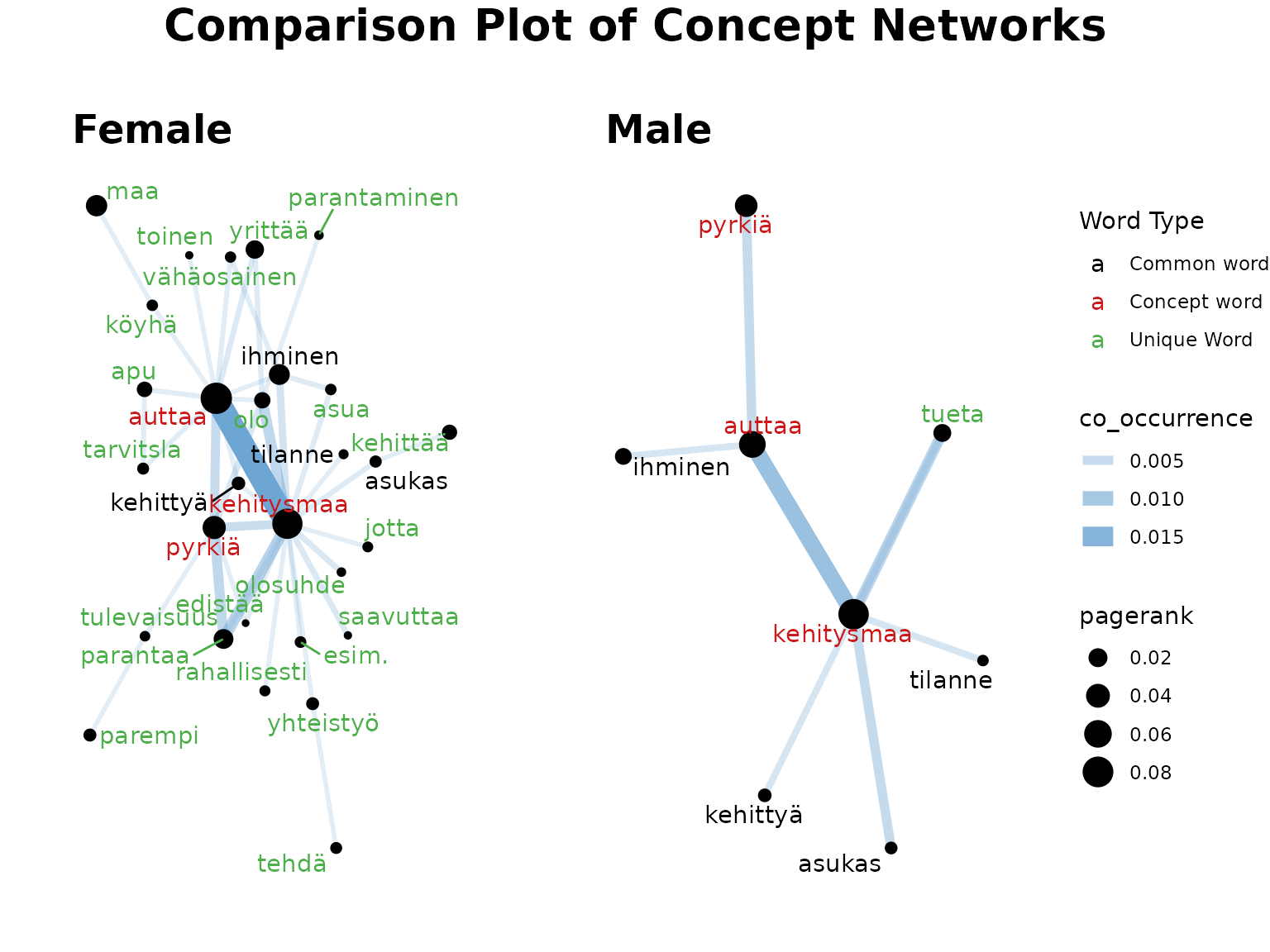

Remarks:

Each of these Concept Networks are created separately, which means that the weights of words are based only on the responses within that gender. Despite this, we have many more words in the female plot (possibly due to there being more responses in this data leading to increased variation). Below, we will run the female with stricter thresholds.

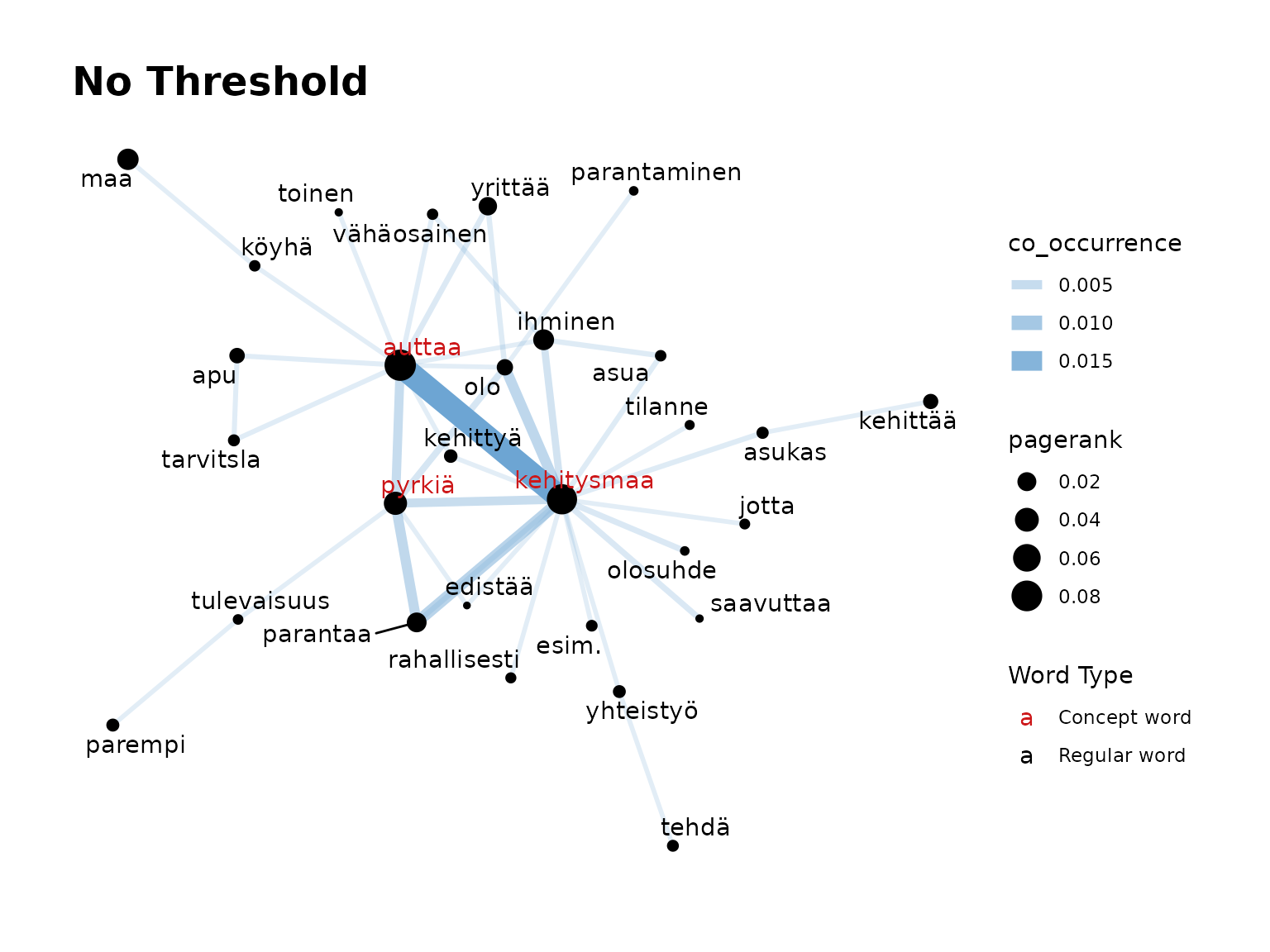
(Note, the threshold works on the RAW count of co-occurences between words, not on the normalised co-occurrence value).

fst_concept_network(female_nltk,
  concepts = "kehitysmaa, auttaa, pyrkiä",
  threshold = NULL,
  title = "No Threshold"
)

fst_concept_network(female_nltk,
  concepts = "kehitysmaa, auttaa, pyrkiä",
  threshold = 5,
  title = "Threshold = 5"
)

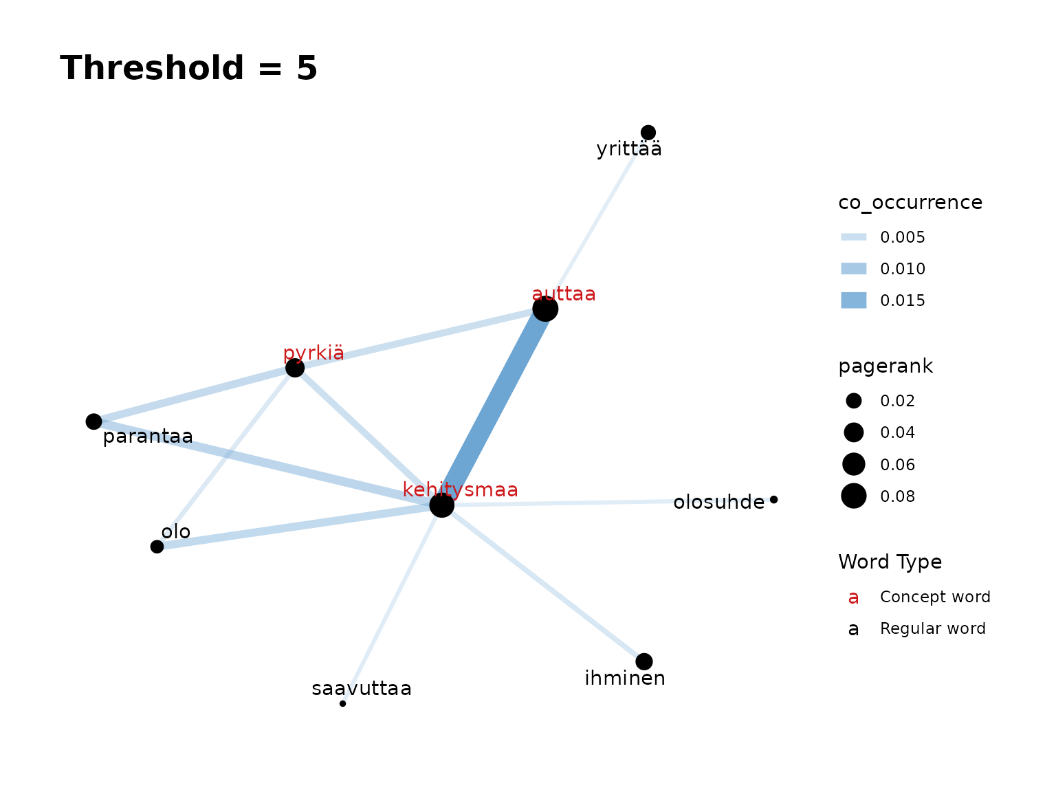
Now let’s manually create the concept networks so that there is a requirement of at least 4 occurrences for words in the female network (there are ~3.7x as many females as males so I have chosen 4). These networks look more comparable now and we can see that the concept networks show different words used around our “concept” words of “kehitysmaa”, “auttaa” and “pyrkiä” by female respondents than male.

concepts <- "kehitysmaa, auttaa, pyrkiä"
female_edges <- fst_cn_edges(female_nltk, concepts, threshold = 4)
male_edges <- fst_cn_edges(male_nltk, concepts)

female_nodes <- fst_cn_nodes(female_nltk, female_edges)
male_nodes <- fst_cn_nodes(male_nltk, male_edges)

min_edge <- min(min(female_edges$co_occurrence), min(male_edges$co_occurrence))
max_edge <- max(max(female_edges$co_occurrence), max(male_edges$co_occurrence))
min_node <- min(min(female_nodes$pagerank), min(male_nodes$pagerank))
max_node <- max(max(female_nodes$pagerank), max(male_nodes$pagerank))

unique2 <- fst_cn_get_unique(female_nodes, male_nodes)

female_cn <- fst_cn_compare_plot(female_edges, female_nodes, concepts,
  unique_lemmas = unique2,
  name = "Female",
  concept_colour = "red",
  unique_colour = "purple",
  min_edge = min_edge,
  max_edge = max_edge,
  min_node = min_node,
  max_node = max_node
)

male_cn <- fst_cn_compare_plot(male_edges, male_nodes, concepts,
  unique_lemmas = unique2,
  name = "Male",
  concept_colour = "red",
  unique_colour = "blue",
  min_edge = min_edge,
  max_edge = max_edge,
  min_node = min_node,
  max_node = max_node
)

fst_plot_multiple(plot1 = female_cn, plot2 = male_cn, main_title = "Comparison Plot of Female and Male Respondences Q11_2")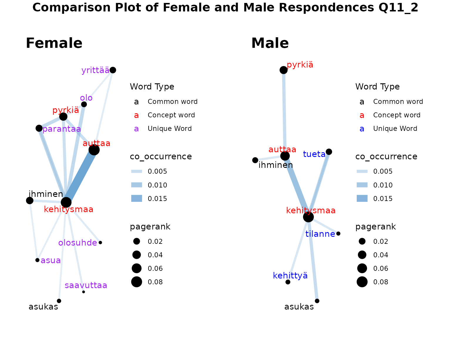

Conclusion

As demonstrated in this tutorial, finnsurveytext contains a number of functions which can be used to compare responses between groups. This analysis could form the start of further work into the responses to question 11_2 by respondents based on their gender, or as just one of many different splits used to investigate the responses.

Citation

Finnish Children and Youth Foundation: Young People’s Views on Development Cooperation 2012 [dataset]. Version 2.0 (2019-01-22). Finnish Social Science Data Archive [distributor]. http://urn.fi/urn:nbn:fi:fsd:T-FSD2821